4. Induction
Note: Some elements of this chapter are still under construction. For examples in Lean for the various types, functions, and proofs defined here, refer to files distributed through git. This chapter will soon be updated with finalized content.
A logic is a formal language in which we use symbolic terms to represent and reason about properties of objects and sets of objects in the world. Until now, we’ve been satisfied to represent objects using terms of only a few types: nat, bool, string, etc.
While these types are essential, their values are not ideal for representing more complex kinds of objects. We’d like to be able to define our own data types, to interpret values as representing more complex objects. Such objects could be quantities in the physical world, such as people, states of machines (e.g., positions or velocities of drones), musical notes. They could also be richer mathematical objects: ordered pairs of objects, lists of objects, trees of objects, sets of objects, sets of pairs of objects, relations between sets, etc.
In this chapter, we see how to define new data types. Once we have a new type, we will then be able to define functions that take or return values of these types. And we will need new principles for logical reasoning about such types, values, and functions. In particular, we will want inference rules that allow us to prove that all objects of a type have a certain property. These are called induction principles. They are introduction rules for universal generalizations over types. Every type comes automatically accompanied by an induction rule for that type.
4.1. Example
Before delving more deeply into general principles and mechanisms, we will illustate the basic ideas by returning to the day type we saw previously in this course. We will repeat it’s definition, show how to define a tomorrow function that takes a day d and returns the next day after d, and prove a simple universal generalization: that for any day, d, seven tomorrows after d is always just d.
4.1.1. A Data Type
To define a new type and its values in Lean, we use an inductive definition. An inductive definition gives a name to a type and defines the set of constructors that can be used to introduce values of the type. When every value of a type is given by a constructor that takes no arguments, we call such a type an enumerated type. It is enumerated in the sense that we give an enumeration (a list) of each of its individual values. As an example, the bool type is an enumerated type. It has just two constant constructors, bool.tt and bool.ff. The day type that we defined in an earlier chapter is also enumerated. It has one constant constructor for each day of the week. Here it is again, in Lean.
inductive day : Type
| sunday : day
| monday : day
| tuesday : day
| wednesday : day
| thursday : day
| friday : day
| saturday : day
We start such a definition with the inductive keyword. The name of our type is day. We declare day to be a type (a value of type, Type). The set of values of this new type is defined by the set of named constant constructors: sunday, monday, etc. Each constructor is constant in that it takes no arguments and by itself is declared to be a value of type, day.
An essential characteristic of inductive data types is that the values constructed by different constructors are different. So no two days as defined here are the same day. Another essential characteristic is that there are no values of a type other than those defined by the available constructors. So the day type as defined here has exactly seven distinct values. We interpret them as representing the real-world days of the week.
4.1.2. Defining Functions by Cases
Give our day data type, we can now define functions that take or return values of the type. We will define a function, tomorrow, that takes a day as an argument and returns the next day of the week.
The behavior of a function when applied to an argument value generally depends on which constructor was used to construct that particular value and what arguments, if any, it was applied to. If the function is applied to a value constructed by the tuesday constructor, for example (which takes no arguments), it should return wednesday. Our objective is to define a type and related functions to model the days of the real-world week.
We specify the behavior of our function by case analysis or pattern matching. Each case has two parts: a matching rule and a result expression. A matching rule specifies a pattern that matches the application of one of the constructors to arguments of the right kinds for that constructor. Names can be given to the arguments. A result expression specifies what result to compute and return when a function application matching the pattern is evaluated.
Because functions in Lean must be total, the set of cases in the definition of a function has to cover all possible function applications. Lean requires that there be a behavior that is specified for every possible application of the function to arguments of the types it takes.
In the simplest of cases, there will be exactly one case for each constructor. When the same behavior is needed for several constructors, these cases can be collapsed into a single rule, as we will see.
To make these ideas clear and concrete we present the definition of a function, tomorrow (we’ll call it tom). It that takes a value, d, of type day as an argument and returns the day after *d*To make the example self-contained, we repeat the definition of the *day type.
inductive day : Type
| sunday : day
| monday : day
| tuesday : day
| wednesday : day
| thursday : day
| friday : day
| saturday : day

def tom : day → day
| sunday := monday
| monday := tuesday
| tuesday := wednesday
| wednesday := thursday
| thursday := friday
| friday := saturday
| saturday := sunday

#reduce tom thursday
#reduce tom (tom friday)
To define a function in this way requires the following steps. Use the keyword, def, followed by the name of the function, followed by a colon, and then the type of the function. Do not include a colon-equals (:=) after the type signature. Then define the behavior of the function by cases, here with one case for each constructor. Each case starts with a vertical bar, followed by the name of the constructor (the matching pattern), then a colon-equals, and finally a result expression that defines the result to be returned in this case. If tom is applied to tuesday, for example, the result is defined to be wednesday.
EXERCISE: Remove one of the cases. Explain what the error message is telling you.
When an expression is evaluated in which tom is applied to an argument, Lean considers each case in the function definition, from top to bottom. Sometimes we get to a point in the case analysis where we don’t care which of the remaining cases holds; we want to return the same result in any case. To do this we specify a pattern that matches several cases. We can use an underscore character as a wildcard in a pattern to match any value of the required type.
Consider, for example, a function, isWeekday, that takes a day and returns a bool, namely tt if the day is a weekday, false otherwise. In the following code, the underscore matches both remaining cases, saturday and sunday. Note also that we do not have to write cases in the order in which they appear in the type definition (where sunday was first).
inductive day : Type
| sunday : day
| monday : day
| tuesday : day
| wednesday : day
| thursday : day
| friday : day
| saturday : day

def isWeekday : day → bool
| monday := tt
| tuesday := tt
| wednesday := tt
| thursday := tt
| friday := tt
| _ := ff
EXERCISE: Find a way to further shorten the text giving the definition of isWeekday by being more clever in the use of wildcard pattern matching.
EXERCISE: Give an inductive definition of a data type, switch, with two values, On and Off (be sure to use upper case O here, as on is a keyword in Lean and cannot be used as an identifier). Define three functions, turnOn and turnOff, and toggle. Each should take and return a value of this type. No matter which value is given to turnOn it returns on. No matter which value is given to turnOff it returns off. The toggle function takes a switch in one state and returns a switch in the other state.
4.1.3. Proofs by Induction
Having seen how to define a type inductively (day) and a function (tom) operating on values of this type, we now turn to the top of induction principles, which are inference rules for proving univeral generalizations about objects of inductively defined types. For example, we might prove that for any natural number, n, the sum of the natural numbers from zero to n is n * (n + 1) / 2.
Associated with each inductively defined type is an associated induction principle. Such a principle is an introduction rule for forall propositions, for universal generalizations/ We use induction rules to construct proofs of propositions of the form forall t : T, P t, where P is a predicate.
When the values of a type are given by a list of constant constructors, as in our preceding example, the corresponding induction principle says that if you have a proof that each value of the type satisfies a predicate, then all values of the type do. The validity of this rule comes from an essential characteristic of inductively defined types: the only values of such types are those that are produced by the available constructors. So if you hve a proof for each constructor then you have a proof for every value of the type; there are no others.
For our day type, and for a predicate P formalizing a property of days, if we have a proof of P sunday and a proof of P monday, and so forth for all the days, then we can deduce that it is the case that forall d, P d. This is the the key idea. Stated formally, the rule is that, for any predicate, P, if you have a proof of P sunday and if you have a proof of P monday and … if you have a proof of P saturday, then you can have a proof of forall d, P d.
For enumerated types, then, a proof by induction is equivalent to a proof by case analysis on the values of the type, with one case for each constructor. The idea is that if you prove a proposition for each of the ways in which an arbitrary value of some type could have been constructed, then you have proven it for all values of that type, because all possible cases are covered.
The strategy of proof by induction is to apply the induction principle to proof argument values to obtain a proof of its forall conclusion. The approach is to do this while leaving the tasks of proving argument proofs (e.g., a proof of P monday) as subgoals.
Let’s start with a proof by induction for our day type. The predicate we will prove is that for any day, d, the day that is seven tomorrows after d is d itself. Formally, we want to prove that,  .
.
We give two versions of the proof. In each case, we first use forall introduction to obtain an arbitrary but specific value, d, of type day. With d as an arbitrary value of this type, we consider all of the ways in which d could have been constructed. That is, we just consider each of the enumerated values that it could possibly have. We do this by using the induction tactic.
The induction tactic gives us one case to be proved for each of the seven constructors. In each case we have to show that tom applied seven times to a particular value, d, returns d itself. These proofs are completed by reduction of the function application expressions and the reflexive property of equality using rfl. Once each case is proved, the universal generalization is proved, and the proof is complete.
inductive day : Type
| sunday : day
| monday : day
| tuesday : day
| wednesday : day
| thursday : day
| friday : day
| saturday : day

open day

def tom : day → day
| sunday := monday
| monday := tuesday
| tuesday := wednesday
| wednesday := tuesday
| thursday := friday
| friday := saturday
| saturday := sunday

example :
    ∀ d : day,
    tom (tom (tom (tom (tom (tom (tom d)))))) = d :=
begin
intro d,
induction d,       -- proof by induction
exact rfl,
exact rfl,
exact rfl,
exact rfl,
exact rfl,
exact rfl,
exact rfl,
end

-- optional material

example :
    ∀ d : day,
    tom (tom (tom (tom (tom (tom (tom d)))))) = d :=
begin
intro d,
induction d,      -- proof by induction
repeat { exact rfl },
end
Optional: Our second version of the proof shows a way to simplying the proof script using what in Lean is called a tactical. A tactical is a tactic that takes another tactic as an argument and that does something with it. Here, the repeat tactical repeats the application of the given tactic (exact rfl) until that tactic fails, which happens when there are no more cases to be proved. We thus avoid having to type the same line seven times as in the first version of our tactic script. In an English language rendition of these formal proofs one would simply say, “each case is proved by simplification and by appeal to the reflexive property of equality.”
EXERCISE: Replace the use of the induction tactic with the use of the cases tactic in each of the preceding proofs. Verify that simple case analysis works. Understand that if you prove that a proposition (such as seven tomorrows from any day is that same day) is proven true for all values of a given enumerated type if it’s proven true for each of them individually.
In this extended introductory example, we have seen (1) the inductive definition of a data type, (2) a function defined by cases, and (3) the proof of a univeral genearalization that establishes that that function has a certain property that it must have if it’s correct. The fact that we can prove it gives us a basis for improved confidence in the correctness of our function definition. We now turn to a deeper exploration and extension of each of these ideas.
The synergistic combination of (1) an inductively defined data type, (2) a set of functions operating on values of such a type, and (3) proofs that such values and functions have key desired properties, establishes one of the most fundamental of building blocks in computer science. We will refer to these combinations as certified abstract data types. An abstract data type combines a data type with operations on values of that type. By certified we mean that proofs are also provided showing that such functions and values have the properties that they must have in order to be correctly defined.
We explore issues that arise in each of these three areas. These issues include the concepts of recursive and polymorphic types, of recursive and polymorphic functions, and the crucial concept of proving universal generalizations by the method of induction. We start with data types.
4.2. Data Types
Many logics, including programming languages (which are specialized logics), and including Lean, support the definition of new data types. Lean supports what are called inductively defined algebraic data types. Such a data type defines a set of values, the values of the type, by defining constructor functions that can be used to construct values of the type. The set of values of a type is then defined to be the set of all and only those values that can be constructed by applying available constructors a finite number of times.
We’ve been using constructor functions all along. The value, tt, in Lean, is one of the two constructors for values of the type, bool, for example. Similarly, succ is a constructor for values of the type, nat. The tt constructor takes no arguments. It is a constant value of type bool. The nat.succ constructor, by contrast, takes one argument, of type nat. A term, nat.succ n, is thus of type nat as long as n is of type nat.
4.2.1. Introduction Rules (Constructors)
A constructor is a simple kind of function. It has a name. It takes zero or more values as arguments. And what it does is to simply bundle up its arguments and label the bundle with the name of the constructor. Such a bundle is then taken to be a term of the specified type.
Constructors are the introduction rules for a give type: they construct values of that type. As an example, and.intro is just a constructor for values of type and S T, where S and T are propositions. As such, and.intro takes two arguments, s of type S (a proof of) S, and, t, of type T. It bundles them up into a term, and.intro s t. We view this term as a bundle labelled and.intro and bundling up s and t. This term is then taken to be of type and S T, and thus to be a proof of the proposition, and S T.
As another example, nat.zero is a one of the two constructors for the type, nat. It takes no arguments. We interpret it as representing the constant, 0. The other constructor for values of type nat is nat.succ. It takes one argument of type nat. The expression, nat.succ nat.zero, is an application of this constructor to one argument. The result is simple the term, nat.succ nat.zero, which you can think of as a bundle with the label, nat..succ and one bundled-up value, nat.zero. This term is taken to be of type nat. This example illustrates the important point that one value of a type can contain smaller values of the same type. Here, for example, the term, nat.succ nat.zero, which is of type nat, contains, or bundles up, nat.zero, which is also of type, nat.
4.2.2. Recursive Data Types
One of the important capabilities in Lean is to define a data type in just this way: so that larger values of a type can contain smaller values of the same type. A value, nat.succ n, of type nat, in this sense contains a smaller value, n, of the same nat type. A list of natural numbers can similarly be seen as either an empty list or as a number (let’s call it the head of the list) followed by a smaller list (let’s call it the tail, or the rest, of the list). The tail, in turn, is of type list, and so itself is either empty or a number (head) followed by an even smaller list (tail).
Recursive data values of this kind are like nested toy dolls. A doll is either the solid doll at the middle (like nat.zero, with no smaller values inside) or it’s a shell doll with another doll inside of it. The doll inside of it could in turn be either solid or another shell. The nesting of shells, however, can only be finitely deep. This is part of the definition of an inductively defined type. What that means is that if one keeps removing shells, then after some finite number of steps, eventually one must reach the solid doll,and at that point the process of peeling off outer shells must terminate.
An inherent characteristic of recursive data types in Lean is that they can be only finitely nested. So, while there is an infinit number of nat values*, for example, each one is finite in size. That is, each has only a finite number of applications of nat.succ to a smaller natural number before one must reach nat.zero. The nat.zero constructor takes no arguments, so it doesn’t bundle up any smaller natural numbers, and the recursion (nesting) ends, or terminates.
Computer science is full of recursive types. As we’ll see soon, we represent lists and trees as values of recursive data types. Even computer programs are just values of recursive data types. For example, a command in Java can be an assignment command, an if then else, or a while command, etc. Each of these is defined by a different constructor. Consider the constructor for an if-then-else command, such as if B then C1 else C2, for example. It bundles a Boolean condition, B, and two smaller commands, C1 and C2, where C1 is to run if the condition is true, and C2, to run otherwise. A bigger if command contains smaller commands inside of it. Of course C1 or C2 could themselves contain even smaller commands. Commands (programs) are thus values of a recursively defined data type. Programs are values of inductively defined data types.
4.3. Functions & Recursion
Once we’ve defined a new type, we can then define funtions that take values of that type as arguments, and that might return values of that type as results. We will now see how we can define functions by case analysis on the possible ways that a given argument might have been constructed. All data values in Lean and in similar languages are values of algebraic data types. A given value will have been constructed by some constructor applied to zero or more arguments.
4.3.1. Elimination (Case Analysis, Pattern Matching)
Whereas constructors provide the means to create objects of given types, functions use objects of given types. When a function is called, it will often have to determine which constructor was used to produce its argument, and what arguments, if any, were given to that constructor when the argument was constructed. This process involves what amount to the use of elimination rules for data types. Just as an elimination rule, such as and.elim_right lets us see what’s inside a proof of a conjunction, so the elimination mechanisms we will meet here allow us to see what’s inside any old data value.
As a simple example, a function that takes a natural number argument and that returns true if that value is zero and false otherwise will have to decide whether the value was construted by the nat.zero constructor ,or by the nat.succ constructor. And in the latter case, it will be essential also to see the value to which the nat.succ constructor was applied to produce the argument.
This examples lead us to the idea that we can define functions by doing case analysis on argument values, with one case for each of the possible forms of an argument. When a function application is evaluated, Lean will then inspect the argument, decide which constructor was used to create it, assign names to the bundled up values (such as the smaller natural number to which nat.succ was applied to construct the value received as an argument), then carry out whatever computation is required for that case. The process of destructuring a value to see how it was built also goes by the name, pattern matching, and is basically elimination for data values.
The following code provides an example. We define a function that takes a value of type nat as an argument and that returns true if it’s zero and false otherwise. It functions by case analysis to determine which constructor was used to produce the argument. If the function is given 0 (nat.zero) as an argument, it returns true. Any other natural number can only have been constructed by applying nat.succ to some value, indicated here by an underscore. If given any such term, the function returns false.
def isZero : ℕ → bool
| nat.zero := tt
| (nat.succ _) := ff

#eval isZero 0
#eval isZero 1
#eval isZero 2
Here is a richer and more interesting example. They key point here is that we can give names to the arguments to which a constructor was applied, and they we can define a return result with an expression that uses those names. Consider a predecessor function: one that takes a natural number, n, as an argument, and that returns zero if n is zero, and that returns the predecessor of n otherwise. It can be defined with two cases. The first case is where n is zero. The second is where n is not zero. In this case, n must be a term of the form nat.succ applied to a one-smaller nat value. That smaller value is what we want to return. Here we give the name n’ that smaller value, and the result that we return in this case is n’. It was essential that we give a name in order to be able to use it to define the desired return result. Study this example carefully.
def pred : ℕ → ℕ
| nat.zero      := nat.zero
| (nat.succ n') := n'

#reduce pred 2
#reduce pred 1
#reduce pred 0
The key points to focus on in this example are two. First, the function is defined by cases, one where the argument was produced by (and is) nat.zero, and one where it was produced by nat.succ applied to a one-smaller natural number. Second, in the second case, we use what is called pattern matching to not only match the name of the constructor, but also to give a name, temporarily, to the value to which that constructor must have been applied. Here we give it the name, n’. We thus match on and give a name to the smaller natural number that is bundled up inside the larger number given as an argument to the pred function. In this way, we gain access to and give a name to the value bundled up inside of the argument value.
4.3.2. Recursion
When data types are recursively defined it is natural, and often necessary, to implement functions that operate on such values recursively. A recursive function applied to a value that contains smaller values of its same type will often call itself recursively to deal with those smaller values.
Now if an argument is recursive in its structure, a function will often itself be defined recursively. When given an argument that contains other values of the same type, it will often call itself to deal with those values recursively. The nesting of function calls then comes to mirror the nesting of values in the argument to which the function is applied.
Here’s a very simple example. The following function takes any natural number, n, as an argument and keeps calling itself recursively with the predecesor of n as an argument until the argument value reaches nat.zero at which point it returns the string, finite.
def finite : ℕ → string
| nat.zero := "finite!"
| (nat.succ n') := finite n'

#eval finite 0
#eval finite 5
#eval finite 100
Consider a more interesting function: one defined to print out all of the elements of a list. Suppose it accepts a value of type, list nat. That list could either be empty, indicated by the constructor, nil; or it could be of the form cons h t, where cons is the name of the second of two constructors, h is the value of type nat at the head of the list, and t, of type list nat, is the rest, or tail, of the list.
The first thing the function has to do is to decide which case holds, and then it needs to function accordingly. If the argument is nil, the function prints nothing and just returns, having completed its job. On the other hand, if the list is of the form, cons h t, then it has something to print: first the value, h, at the head of the list, and then, t, the rest of the list.
The wonderful, almost magical trick, is that to print the reset of the list, the function can just call itself, passing t (the smaller list contained within the argument list) as an argument. If you trust that that function is correctly implemented, then you can trust that it really will print the rest of the list, and you need think no further about the nested function calls. You think: to print the list, we first print the head, then *recursively print the tail.* That’s it!
4.3.2.1. Structural Recursion
Because any value of type list nat is finitely deeply nested, with nil as the so-called base case, such a list-printing function is guaranteed to reach the nil list, and thus to terminate, within a finite number of steps. We saw the same principle at play in the simple function, finite. No matter how large a value of type nat we give it, it will eventually reach nat.zero, terminate, and return the string, “finite!”.
This kind of recursion is called structural recursion. It is of deep importance in the theory of programming, because it allows one to immediately know that a recursive function will terminate. Knowing that a function always terminates, in turn, is essential to ensuring that a function is total, i.e., that it will return a value for any value of its argument type. If a function could go into an infinite loop, then it would fail to return a result for some values. That, in turn, for reasons we have not yet explained, would make its logic inconsistent. Lean will thus not accept such a non-terminating function definition.
Not all recursive functions terminate. Here’s an example. Consider a function called badnews that takes a natural number, n, as an argument, returns a proof of false, and works by simply calling itself with n as its argument. Such a function once called will never return. It does not pass a smaller part of n as an argument. It goes into an infinite regress, calling itself again and again always with the same argument.
If such a function were allowed to be defined in Lean, then the function application expression, (badnews 0), would be a term of type false (because that’s the return type of the function)! Allowing such a function would make Lean’s logic inconsistent. Such functions must therefore not be allowed to be defined and Lean will reject them. On the other hand, Lean recognizes that structurally recursive functions will always terminate, and it will accept them without any further proof of termination.
4.3.2.2. Generative Recursion (Optional)
Every function in Lean must be guaranteed to terminate. All structurally recursive functions are guaranteed to terminate, so structural recursion is very useful. There are recursive functions that do terminate but that are not structurally recursive. For such functions, explicit proofs that they terminate must be given before Lean will accept them as valid.
For example, a method for sorting the values of an array into increasing order might work by partially rearranging the elements of the array in a certain way, then recursively doing the same thing for each half of the resulting array. One sorting algorithm of this kind is called Quicksort. The problem is that these sub-arrays, having been rearranged, are no longer substructures of the original array. The resulting algorithm is recursive but not structurally recursive.
This kind of recursion is called generative recursion. It can be seen and argued that this recursion will always terminate, because at each step a finite-length array is reduced to haf its original size, and the size of the arrays being passed as arguments to recursive calls keep getting smaller, and they eventually reach size one, at which point the recursion would stop. So even though the recursion is not structural, something is getting smaller on each recursive call, and that something (the array size) eventually reaches a minimum value, at which point the recursion terminates. We say that such a recursion is well founded. To get Lean to accept an algorithm that uses generative recursion you must provide a separate proof of termination. Indeed, when programming in general, whenever you use recursion, you must be able to make a valid argument for termination in all cases.
To do this, you have to show that some value gets smaller each time the function is called, and that that value will, after some finite number of steps, reach a least value, a base case, beyond which the recursion cannot continue. Doing this is hard in general. In fact, there are generative recursions for which it is not known whether they terminate (for all inputs) or not!
One example is that of the so-called hailstone function. It takes a natural number, n, as an argument. If n is even, the function calls itself recursively with the value, n/2. If n is odd, the function calls itself recursively with the value, n * 3 + 1. Given 5 as an argument, for example, this function calls itself recursively with the following values: 16, 8, 4, 2, 1. We refer to this sequence of argument values as the hailstone sequence for the value 5. When such a sequence reaches 1, if it does, then it is done. With the value 7 as an argument, the hailstone sequence of values it calls itself on are: 22, 11, 34, 17, 52, 26, 13, 40, 20, 10, 5, 16, 8, 4, 2, 1.
As you can see, the value of the argument to the recursive call can fall for a bit and then be pushed way back up again, like a hailstone in a storm cloud. What is unknown is whether such sequences terminate for all values of n. It remains a possibility that for some values, the hailstone never reaches the ground. We have neither a proof of termination, nor of non-termination of this function for all natural number arguments.
The recursion in this case is generative. It certainly isn’t structural: n * 3 + 1 is in no way a substructure of n. Because there is no known proof of termination, the hailstone function cannot be implemented as a function in Lean, as the following code demonstrates. To ensure that the logic of Lean remains consistent, Lean will not accept such a definition. Be sure to look closely at the error message. It basically says, “I, Lean, can’t see that this function always terminates, and you didn’t give me an explicit proof that it will terminate, so I will not accept it as a valid function definition.”
def hailstone : nat → true
| nat.zero := true.intro
| (nat.succ nat.zero) := true.intro
| n :=  if (n % 2 = 0) then
            (hailstone (n/2))
        else
            (hailstone (n*3+1))
EXERCISE: Implement this function in Python but have it return the number of times it called itself recursively for a given argument value, n. Add a driver function that runs your program for values of n ranging from 1 to, say, 100 (or to any other number, given as an argument). Have you program output a bar chart showing the number of recursive calls for each such value of n.
4.3.2.3. Co-Recursion (Optional)
Optional: As an aside for the interested student, Lean does support what are known as co-inductive types. Such types can be used to represent values that are infinite in size. In particular, co-inductive types can represent inifinite-length streams of values produced by continually iterated applications of specified procedures. Such types are typically used to represented processes that are not necessarily guaranteed to terminate. Examples include games that a user might never win or lose, and an operating system that is meant to keep running until someone shuts it down, which might never happen. The logical principles for reasoning with co-inductive types are more complex than those for reasoning with inductively defined types.
4.4. Induction
When one defines a new type, T, a new reasoning principle is needed to allow one to prove universal generalizations concerning values of the new type. That is, one has to be able to prove propositions of the form, forall t : T, P t, where P is some predicate and T is the new type of interest. Associated with each inductive type is a type-specific inference rule called an induction principle. The application of such a rule to construct a proof of forall t : T, P t is commonly known as the strategy of proof by induction.
Some students might have already seen what is called proof by mathematical induction. This is simply the application of the induction principle for the type of natural numbers. The concept of proof by induction is much broader. It applies to any type of values. In computer science, it can be used to prove propositions about natural numbers, lists, trees, computer programs, or any other inductively defined type. Every inductively defined data type comes with its own induction principle.
When a type has only a finite number of values, the induction principle for that type states that if you prove that each value of a type has some property, then all values of that type have that property. This amounts to a proof by case analysis of the values of the type. If one shows that a given predicate is satisfied by each individual value in the finite set of values of a type, then it is clearly true for all values of that type.
The challenge comes when one considers recursive types, such as nat. What an induction principle then says is that (1) if you can prove that all of the base constructors of the type satisfy P, and (2) if whenever the arguments to a recursive constructor satisfy P, then the values produced by the constructor also satisfies P, then (3) all values of the type satisfy P.
To prove forall n : nat, P n, for example, one first proves P nat.zero, i.e., one proves that zero, a base constructor, has the specified property. Then one shows, for the second constructor, that if n satisfies P then nat.succ n also satisfies P. With these two proofs, you can then conclude that every value, n of type nat&, satisfies *P. This is a proof by induction. Zero has the property, by the first case, then one does by the second case, and because one does then by the second case, so does two as well, then by the second case again so does three, and so it goes ad infinitum.
Now we can see the formal induction principle for the type, nat. For a given predicate, 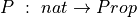 , to prove
 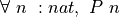 , we must prove (1)
  , and (2)
  . The induction principle just expresses this idea as one big rule, which, in English says, for any predicate, P, if P 0, then if also (P n implies P (n + 1)) then forall n, P n. Formally, it’s
  .
.
An induction principle is an introduction rule for universal generalizations. To prove the universal generalizations that is the conclusion of the rule, it suffices to prove both of the premises. The rule, in other words, takes proofs of the premises as arguments and gives back a proof of the universal generalization as a result. A proof of the first premise, the base case, establishes that the predicate is true for zero. The proof of the second preise establishes that if it’s true for any value, n, then it must be true for the next larger value, nat.succ n. If both conditions are true, then by the first condition it’s true for zero, so by the second condition it must also be true for one; but because it’s true for one, then again by the second condition it must be true for two; and then for three; and so on, ad infinitum. Therefore it is value to conclude that it’s true for every natural number.
Reading the induction rule from right to left indicates that if you want to prove the forall, then it suffices to prove the premises, P 0 and P n implies P (n + 1). This is the strategy of proof by induction for the natural numbers. One applies the induction principle, leaving the proofs required as arguments as sub-goals. Here’s the rule for nat in inference rule notation.
Todo
add inference rule notation
Other recursively defined types have analogous induction rules. The induction principle for lists, for example, says that if you prove that a predicate is satsified by the empty list, and if you prove that whenever it’s satified by any list it’s then also satisfied by any one-larger list, then it’s satsified by all lists. If there are only a few things that one remembers from this course, one of the good ones would be to remember that proof by induction is a general method that can be used with values of any inductively defined type.
4.5. Parameterized Types
The type definition facilities of Lean and of similar logics also support the definition of parameterized, or polymorpic, types. Just as predicates are propositions with parameters, polymorphic types are types with parameters. And just as we represent predicates as functions that take arguments and return propositions, we represent polymorphic types as functions that take other values (often types) as parameters and that return types.
It sounds complicated but it’s not really. Consider as an example a type, list nat, the type of lists of natural numbers. One value of this type would be the list, [1, 2, 3]. The type, list bool, by contrast, is the type of lists of Boolean values. A value of this type would be [tt, tt, ff]. The type, list string, is the type of lists of strings. Indeed, for any type, T, list T is the type of lists containing elements of type, T.
We can thus say that list, is a parameterized, or polymorphic, type. Of course list isn’t really a type, per se. Rather, it’s a function that takes a type, such as nat or bool or string as an argument, and that returns a type, such as list nat or list bool or list string. Such a type-building function is sometimes called a type constructor. This use of the term, constructor, differs from that above, where a constructor is a function for producing values of a given type. A type constructor by contrast takes arguments and gives back a type.
Here’s a very simple example of a polymorphic type. We’ll call it box T. A value of this type does nothing but contain a value of type T. Along with the polymorphic box type we also define a function that uses pattern matching to extract and return the content of any box.
inductive box { T : Type }
| pack : T → box

def unbox : ∀ { T: Type }, @box T → T
| T (box.pack t) := t

def box1 := box.pack 3
def box2 := box.pack ff

#eval unbox box1
#eval unbox box2
There are several syntactic aspects of this example to study. First, we define the box type as taking a type argument, T, and we specify that this argument is implicit, as it will be possible in most cases to infer T from the argument to pack. Second, box has just one constructor, pack. As a constructor function, pack takes T as an implicit argument. It then takes a value of type T as an explicit argument and returns a box that conceptually contains that value.
When a data type is polymorphic, then the functions that deal with values of that type must also be polymorphic. All that really means is that they have to take corresponding types as arguments. This will usually be done implicitly. As an example, a function, print_list, to print values of A type, list T, would take two arguments: a type, T, and a value of type list T. In most cases, T will be an implicit argument so that one doesn’t have to specify it explicitly each time one applies the print_list function to a given list argument.
These ideas are illustrated in our unbox function. Being a function on values of a polymorphic type, is also polymorphic: it takes a type argument, T, albeit implicitly. We use a forall here to give a name to this argument. After the comma, we define the rest of the type of this function. It takes an explicit argument of type box T and returns a value of type T. The @ tells Lean to let us give the implicit type argument to box explicitly. Finally, even though the unbox function takes T implicitly, it has to be explicit in the pattern matching. It is also important to remember that constructor expressions in pattern matching rules need to be enclosed in parentheses when they take arguments.
EXERCISE: Define a polymorphic type, option T, where T is a type parameter. This type will have two constructors. The first will be called none and will be a constant of type option T. The second will be called some and will take (and will box up) a value of type T, just like the box type does. Values of an option type can be used to represent either a good return value, some t, from a function, or an error, none.
EXERCISE: Define a new predecessor function for natural numbers. When applied to zero, this function should return a value, none, of type option nat. In all other cases, it should return some n’, where n’ is one less than the given argument. Using option types is one important way to represent partial functions in a language such as Lean. The function is total in that it always returns an option value, but in some cases that value represents a defined result, and in other cases (none), an undefined result.
The rest of this chapter illustrates how these ideas, of data types, function definition by cases, and proof by induction, play out in the definition of a range of fundamental abstract data types. These include polymorphic pairs, the natural numbers, lists, and trees.
4.6. Polymorphic Pairs
Our first extended example is that of a polymorphic data type for representing ordered pairs, where the types of the elements of an ordered pair are type parameters of our polymorphic type. Examples of ordered pairs include (1, 2), an ordered pair of natural numbers; (tt, ff), an ordered pair of Boolean values; and (1, tt), and ordered pair whose first element is a natural number and whose second element is Boolean. That is the data type.
Our data type will be polymorphic in the sense that a pair is a value of an inductively defined data type that takes the types of the first and second elements of a given pair as parameters. Our type will be polymorphic in just this sense. Our aim is to give a complete example with a data type, functions, and statements and proofs of properties. We discuss each element below.
4.6.1. Inductive Data Type
A polymorphic inductive data type is a data type with parameters. Such a “type” actually defines a whole family of data types, one for each combination of parameter values. We use the term, type constructor for a polymorphic type. In Lean, prod is a type constructor with two parameters, each a type. Values of type prod S T represent ordered pairs in which the first element is of type, S, and in which the second element is of type, T. Here we replicate Lean’s prod type, calling it myprod here to avoid naming conflicts with Lean’s built-in libraries.
/-
Data type
-/

inductive myprod (S T : Type) : Type
| mk (s : S) (t : T) : myprod

-- it works
#check myprod nat string

-- a value; type parameters to constructors are inferred
def aPair :
    myprod nat string :=    -- type
    myprod.mk 1 "Hello"     -- value

/-
Functions
-/

/-
Our first two functions are "getter" functions
for the first and second components of a pair,
respectively. These are basically "elimination"
rules, as they give access to the insides of a
pair. We give each function definition without
and then with implicit type parameters. As you
will see, it's easier to use the versions that
have implicit parameters.
-/
-- Without implicit type parameters
def fst' : ∀ (S T : Type), myprod S T → S
| S T (myprod.mk f s) := f

-- With implicit type parameters
def fst : ∀ { S T : Type }, myprod S T → S
| S T (myprod.mk f s ) := f

-- Without implicit parameters
def snd' : ∀ (S T : Type), myprod S T → T
| S T (myprod.mk f s) := s

-- With implicit parameters
def snd : ∀ { S T : Type }, myprod S T → T
| S T (myprod.mk f s) := s

/-
Our third and last function takes a pair and
returns a pair with the values swapped.
-/
-- Without implicit parameters
def swap' : ∀ (S T : Type), myprod S T → myprod T S
| S T (myprod.mk f s) := (myprod.mk s f)

-- With implicit parameters
def swap : ∀ { S T : Type }, myprod S T → myprod T S
| S T (myprod.mk f s) := (myprod.mk s f)

-- examples without implicit parameters
#eval fst' nat string aPair
#eval snd' nat string aPair
#eval swap' nat string aPair

-- examples with implicit parameters (better!)
#eval fst aPair
#eval snd aPair
#eval swap aPair

#check swap aPair       -- Note the type!


/-
Properties
-/

/-
Getters followed by constructor gives same pair.
-/
theorem proj_ok' :
∀ (S T : Type) (p : myprod S T),
    myprod.mk (fst p) (snd  p) = p :=
begin
intros S T pr,
cases pr with f s,
exact rfl,
end

/-
Swapping twice gives back starting pair.
Note that you *must* "eliminate" using
cases before rfl will work.
-/
theorem swap_involutive :
    ∀ (S T : Type) (p : myprod S T),
    swap (swap p) = p :=
begin
intros S T p,
cases p,
exact rfl,
end
The name of our type is myprod. This type type takes two other types, S and T, as arguments. These become the types of the first and second elements of any pair of type myprod S T. Consider, for example, myprod nat nat. In this term, the type constructor, myprod, is applied to two values of type, Type, namely nat and nat, yielding the type myprod nat nat. Check its type by launching the preceding example in your browser.
This type is a type whose values represent ordered pairs of natural numbers. Similarly, myprod bool bool, is our type for representing Boolean pairs. And myprod string bool is the type of pairs whose first elements are of type string and whose second elements are of type bool.
The second line defines mk as the one available constructor for values of this type (these types). The only way to create a value of type myprod S T is to use this constructor (or to use a function that uses it directly or indirectly). It takes two values: one of type S, and one of type T. Applying it to two values, s : S and t : T, yields a term, myprod.mk s t. We take it to represent the ordered pair, (s, t) of type, myprod S T.
A type, myprod S T, is called a product type. The values of such a type are pairs whose elements are of the corresponding types. Lean’s libraries define the type constructor, prod for defining product types, a nice cross product notation for representing product types, and a nice ordered pair notation for representing values. Check it out.
#check prod nat nat
#check prod bool bool
#check prod string bool

#check ℕ × ℕ
#check bool × bool
#check string × bool

example : ℕ × ℕ := (1, 2)
example : bool × bool := (tt, ff)
example : string × bool := ("Hello", tt)
We will skip defining such notations for myprod, so that you can see more directly what’s going on behind such notations.
Next we give four examples of ordered pairs using our myprod type constructor. What is nice to see is that we can define pairs with different types of first and second elements. Lean infers the types from the arguments given to the constructor. Look at the results of the #check commands. You will see that pairs are of different types, varying in the types specified by S and T.
We that that a “type” that takes other types as arguments is polymorphic. If we check the type of myprod, we see that it’s not really a type at all. It’s a value of type, Type to Type to Type. It’s a function that takes two types, call them S and T, as arguments, and that returns a type, myprod S T, as a result. This function represents a parameterized type, in the same way a function can represent a predicate, a parameterized proposition. We call myprod a type constructor. We have thus defined not just a single pair type, but a whole, indeed infinite, family of pair types, one for each combination of first and second element types.
4.6.2. Functions
The second component of a certified abstract data type is a set of functions that operate on values of the given type. We now define three functions for this type. The first function, fst, is the first element projection function. When applied to a pair it returns the first element of the pair. The snd function is similar but it returns the second element of the given pair. The third function, rev, takes a pair and returns it but in the reversed order.
Like the type itself, these functions are polymorphic in the sense that they take apply to values of a polymorphic type. In specifying these function, we indicate that these type arguments should be implicit by using curly braces. Lean will be able to infer the types, S and T, from the type of a the pair given as an argument.
Our product type has just one constructor, so there is just one case to consider in the definition of each of these functions: the case where a pair was constructed by applying myprod.mk to two types and to values of each of the types. The pattern matching construct that we use to define each case not only determines what constructor constructed the value being inspected; it also assigns names the arguments to which that constructor was applied. We thus get names for the parts from which an object was constructed.
What we see here is closely related to what happens when we apply the cases tactic in a proof script. When applied to a proof of a disjunction, for example, it gives us names for the assumed proofs in each case. When applied to a proof of conjunction, it does the same. When applied to a proof of an existential, it does the same. Pattern matching is an elimination construct: it throws away the constructor but gives us the pieces to which it was applied with names for each piece. The fst function destructures a pair and returns its first element; snd destructures a pair returns its second element; rev destructures a pair to obtain its parts and then constructs a new pair by applying mk (an introduction rule for our type) to the elements of the given pair in the opposite order. This precisely the use of an elimination principle followed by an introduction principle. Constructors are introduction rules for a given type.
inductive myprod (S T : Type) : Type
| myprod.mk (s : S) (t : T) : myprod

open myprod

def fst : ∀ (S T : Type), (myprod S T) → S
| S T (myprod.mk s t) := s

def snd : ∀ (S T : Type), (myprod S T) → S
| S T (myprod.mk s t) := t

def rev { S T : Type } (p : myprod S T) : myprod T S :=
    myprod.mk (snd p) (fst p)

-- let's test to see if it all works
#check (myprod.mk 1 ff)
#check fst (myprod.mk 1 ff)
#check snd (myprod.mk 1 ff)
#check rev (myprod.mk 1 ff)
#check rev (rev (myprod.mk 1 ff))
#reduce fst (myprod.mk 1 ff)
#reduce snd (myprod.mk 1 ff)
#reduce rev (myprod.mk 1 ff)
#reduce rev (rev (myprod.mk 1 ff))
After the definitions of the three functions, we exercise our data type and its functions by checking the types of various terms using our functions.
4.6.3. Properties
The final component of a certified abstract data type is a set of proofs of properties involving functions and values of the type. We show that, as we have coded it, our abstract data type has two specific and desired properties: first, if we take a given pair apart and then put it back together from the pieces, we just get back the given pair. Second, we show that rev, is involutive. That means that if one applies it twice to a value, the result is that same value. We tested this proposition in the preceding example by confirming that it’s true for one particular case. Here we prove beyond any doubt that it’s true for all pairs that might ever be constructed, with any existing or future types as element types; so we no longer need to test our code. It is proven.
inductive myprod (S T : Type) : Type
| mk (s : S) (t : T) : myprod

def fst' : ∀ (S T : Type), myprod S T → S
| S T (myprod.mk f s) := f

def p1 := myprod.mk "Hello" tt
#check p1

#eval fst' string bool p1

def fst : ∀ { S T : Type }, myprod S T → S
| S T (myprod.mk f s ) := f

#eval fst p1

def snd' : ∀ (S T : Type), myprod S T → T
| S T (myprod.mk f s) := s

def snd : ∀ { S T : Type }, myprod S T → T
| S T (myprod.mk f s) := s

def swap' : ∀ (S T : Type), myprod S T → myprod T S
| S T (myprod.mk f s) := (myprod.mk s f)

def swap : ∀ { S T : Type }, myprod S T → myprod T S
| S T (myprod.mk f s) := (myprod.mk s f)

#eval swap p1
#check swap' string bool p1

theorem proj_ok :
    ∀ (S T : Type) (s : S) (t : T),
    myprod.mk
        (fst (myprod.mk s t))
        (snd (myprod.mk s t)) =
    (myprod.mk s t) :=
begin
intros S T s t,
exact rfl,
end

theorem proj_ok' :
    ∀ (S T : Type) (pr : myprod S T),
    myprod.mk
        (fst pr)
        (snd  pr) =
    pr :=
begin
intros S T pr,
cases pr with f s,
exact rfl,
end

theorem swap_involutive :
    ∀ (S T : Type) (pr : myprod S T),
    swap (swap pr) = pr :=
begin
intros S T pr,
exact rfl,      // fix this proof
end
EXERCISE: Write some code creating a few values of the myprod type (for different type parameter values), then write some code applying both forms of function definitions to some of those values, with and without use of explicit parameters.
Proving theorems about one’s abstract data types not only gives one confidence that they are right. It can also justify certain decisions by users of such types. For example, if some client codehad a term, (rev (rev p)), the involution theorem justifies replacing it with just p, reducing code complexity and possibly improving runtime performance.
Compiler writers develop many complex and subtle optimizations of this sort. Knowing that optimized code is equivalent to unoptimized code is a major challenge. Bugs in compilers are a significant concern when the failure of compiled code to behave as specified in the source code could have unacceptable consequences. The techiques you are learning have been applied in the development, by Prof. Appel at Princeton, of a certified C compiler. It comes with a proof that for all C programs, the compiled and optimized code produced by this compiler has exactly the same meaning as the C source code itself.
4.7. Boolean Algebra
In this section of this chapter, we develop a CADT for Boolean algebra. You’re familiar with Boolean algebra from your earlier work in programming. The aspects to focus on here are how a Boolean data type is defined; how Boolean functions are defined (by case analysis); and how theorems can be stated and proved by induction.
inductive mybool : Type
| ttt : mybool
| fff : mybool

open mybool

-- unary functions (why four?)

def id_mybool (b: mybool) : mybool := b
def true_mybool (b: mybool) := ttt
def false_mybool (b: mybool) := fff
def not_mybool: mybool → mybool
| ttt := fff
| fff := ttt

-- binary functions (how many are there total?)

def and_mybool: mybool → mybool → mybool
| ttt ttt := ttt
| ttt fff := fff
| fff ttt := fff
| fff fff := fff

def or_mybool: mybool → mybool → mybool
| ttt ttt := ttt
| ttt fff := ttt
| fff ttt := ttt
| fff fff := fff

-- using wildcards to match multiple cases
def or_mybool': mybool → mybool → mybool
| fff fff := fff
| _ _ := ttt

-- truth table for not and (nand) using wildcards
def nand_mybool: mybool → mybool → mybool
| ttt ttt := fff
| _ _ := ttt

-- we can also implement nand using what we already have
def nand_mybool' (b1 b2 : mybool) : mybool := not_mybool (and_mybool b1 b2)

def nor_mybool (b1 b2 : mybool) : mybool := not_mybool (or_mybool b1 b2)

def xor_mybool: mybool → mybool → mybool
| ttt ttt := fff
| ttt fff := ttt
| fff ttt := ttt
| fff fff := fff

def implies_mybool: mybool → mybool → mybool
| ttt ttt := ttt
| ttt fff := fff
| fff _ := ttt

-- bi-implication as conjunction of implications
def iff_mybool (b1 b2 : mybool) :=
and_mybool
        (implies_mybool b1 b2) (implies_mybool b2 b1)

-- certificates

-- not is involutive
theorem involutive:
    ∀ b : mybool, not_mybool (not_mybool b) = b :=
begin
    intro b,
    cases b,
    apply rfl,
    apply rfl,
end


-- and is commutative
theorem and_mybool_comm :
    ∀ b1 b2 : mybool, and_mybool b1 b2 = and_mybool b2 b1 :=
begin
intros b1 b2,
induction b1,
induction b2,
trivial,
trivial,
induction b2,
trivial,
trivial,
end

// (and b1 b2) impies (or b1 b2)
theorem and_mybool_implies_or_mybool :
    ∀ b1 b2 : mybool,
        implies_mybool (and_mybool b1 b2) (or_mybool b1 b2) = ttt :=
begin
_               -- exercise
end


theorem demorgan1 : ∀ b1 b2 : mybool,
    not_mybool (and_mybool b1 b2) =
    or_mybool
        (not_mybool b1)
        (not_mybool b2) :=
begin
_               -- exercise
apply rfl,
end

theorem demorgan2 : ∀ b1 b2 : mybool,
    not_mybool (or_mybool b1 b2) =
    and_mybool
        (not_mybool b1)
        (not_mybool b2) :=
begin
_               -- exercise
end
4.7.1. Data type
The name of our type is mybool so as not to conflict with the bool type imported automatically from Lean’s librarues. Like day, our mybool type is an enumerated type. The constructors simply enumerate the finite number of constant values of the type. Our type has just two constructors, ttt and fff. They correspond to the two tt and ff constructors of Lean’s official bool type.
4.7.2. Functions
With this data type in hand, we now specify the functions of the abstract data type.
We start with unary functions, of type  A unary function takes one argument of type mybool and return a value of this same type. One example is the Boolean not function. Only four such functions can be defined. We then move on to binary functions, of which there are sixteen. Examples include Boolean and, or, and implies.
First we present an implementation of the Boolean and function. Applied to Boolean true and true it must return true, and in all other cases it must return false. The new construct we see in this example is matching on two arguments. The four possible combinations of the two possible values of each of b1 and b2 are the cases we must consider. As for syntax, note the comma between the arguments of the match keyword, and the commas between constructor expressions in the individual cases.
We notice that all of the combinations of input values after ttt and ttt return fff. We can use a “wildcard” in a match to match any value or combination of values. Matches are attempted in the order in which rules appear in code.
EXERCISE: Why is it important to try to list the ttt, ttt case before giving the wildcarded rule? Explain.
EXERCISE: Implement each of the following Boolean operators: or (or_mybool), implies (implies_mybool)
Exercise: A binary Boolean operator takes two Boolean values as arguments and returns a Boolean value as a result. Explain why there are exactly 16 functions of this type.
4.7.3. Properties
If you’ve implemented the operations we have asked for, then you should be ready to express and prove that your function implementations has the properties expected of the corresponding real Boolean functions.
For example, we’d expect Boolean conjunction to be commutative. We could try out a few test cases and then hope for the best, or we can state and prove as a theorem the proposition that it’s commutative. We now do the latter.
Notice that we start with induction on b1. This does a case analysis on the possible values of b1. Within the consideration of the first case, we do induction on b2. That gives us two sub-cases within the first case for b1. Once we’re done with this first case, we turn to the second case for b1. We use induction on b2 again, to consider the two possible cases for b2 in the context of the second case for b1.
We address four cases in total. We show in each case, that the proposition (that and commutes) is true. There are no other cases, and so we have proved that it is true for all cases, thus for all possible values of b1 and b2. The universal generalization is thus proven. The proof is by what we call exhaustive case analysis. We check each and every case and thereby “exhaust” all of the possibilities.
Next is a second example. We prove that one of DeMorgan’s two laws, about how not distributes over and, holds for our implementation of Boolean algebra. If it doesn’t hold, look for bugs in your code. If it does, that should increase your confidencce that you’ve got a correct implementation. Proving that all of the expected properties of Boolean algebra hold would be proof positive that you have a correct implementation. You’d then have a certified abstract data type for Boolean algebra.
EXERCISE: Formally state and prove the other of DeMorgan’s Law for Boolean algebra.
EXERCISE: Formally state and prove the proposition that (and b1 b2) implies (or b1 b2). Give a proof by induction.
EXERCISE: Implement the Boolean equivalent operator, then use it to write a proposition asserting that for all Boolean values, b1 implies b2 is equivalent to not b2 implies not b1.
EXERCISE: Try to prove the related proposition that for all Boolean values, b1 implies b2 is equivalent to not b1 implies not b2. What scenario makes it impossible to complete this proof?
EXERCISE: Implement all sixteen binary operations in Lean, using mybool to represent the Boolean values. Name your functions in accordance with the names generally used by logicians, but add “_mybool” at the end, as we’ve done for and.
EXERCISE: Do some research to identify the full set of properties of operations in Boolean algebra. Formalize and prove propositions asserting that your implementation also has each of these properties.
4.8. Natural Numbers
The real power of proof by induction becomes evident when we define constructors for a type that take “smaller” values of the same type as arguments. This is the case for the type, nat, and for many other data types, including lists, trees, and computer programs.
In this section, we consider a data type for representing natural numbers. In short, we show you how the nat type is defined. We then develop a set of basic arithmetic functions, such as addition, using this representation. Finally we formulate and prove propositions to show that our implementation has properties required of a valid implementation of natural number arithmetic.
inductive mynat : Type
| zero : mynat
| succ : mynat → mynat

-- functions

-- some unary functions
def id_mynat (n: mynat) := n
def zero_mynat (n: mynat) := mynat.zero
def pred : mynat → mynat
| mynat.zero := mynat.zero
| (mynat.succ n') := n'

-- a binary function, and it's recursive
def add_mynat: mynat → mynat → mynat
| mynat.zero m := m
| (mynat.succ n') m :=
    mynat.succ (add_mynat n' m)

-- a certificate

-- zero is a left identify
theorem zero_left_id :
    ∀ m : mynat, add_mynat mynat.zero m = m :=
begin
intro m,
trivial,
end

-- zero is a right identity, requires induction
theorem zero_right_id :
    ∀ m : mynat, add_mynat m mynat.zero = m :=
begin
intro m,
-- proof by induction
induction m with m' h,
-- first the base case
apply rfl,
-- then the inductive case
simp [add_mynat],
assumption,
end
4.8.1. Data Type
The crucial difference in this example is that it involves a constructor that allows larger values of our natural number type (we’ll call it mynat) to be built up from smaller values of the same type. What we can then end up with are terms that look like Russian dolls, with smaller terms of one type nested inside of larger terms of the same type. Just consider again the way that the natural number, $3$ is represented: as the term, nat.succ 2, where 2 in turn is represented as nat.succ 1, and where 1 is represented as nat.succ nat.zero. We see that nat.zero, being a constant, allows for no further nesting. It is what we will call a base case.
namespace mynat

inductive mynat : Type
| zero : mynat
| succ : mynat → mynat
Our type is called mynat. It has two constructors. The first, mynat.zero, is a constant constructor. It takes no arguments. The second, mynat.succ, is parameterized: it takes a “smaller” value, n, of type mynat, as an argument, and constructs a term, mynat.succ n, as a result; and this term is now also of type mynat.
Given this definition, we can construct values of this type, either using the mynat.zero constructor, or by applying the mynat.succ constructor to any term of type mynat that we already have in hand.
namespace mynat

inductive mynat : Type
| zero : mynat
| succ : mynat → mynat

-- we give nice names to a few terms of this type
def zero := mynat.zero
def one := mynat.succ mynat.zero
def two := mynat.succ one
def three :=
    mynat.succ
        (mynat.succ
            (mynat.succ
                zero))
def four := mynat.succ three

#reduce one
#reduce two
#reduce three
#reduce four
We see something very different in this example than in the previous examples of enumerated and product types: larger values of a type, here mynat, can be constructed from smaller values of the same type. Terms of such a type have what we call a recursive structure. Eventually, any such recursion terminates with a non-recursive constructor. We call such a constructor a base case for the recursion.
EXERCISE: Define similarly named terms for the values five through ten. Write the term for seven as seven applications of mynat.succ to mynat.zero, to be sure you see exactly how the succ constructor works.
EXERCISE: Define a type called nestedDoll. A nestedDoll is either a solidDoll or it is a shellDoll with another nestedDoll that we think of as being conceptually inside of the shell.
4.8.2. Functions
Given our new data type, we can now define functions that take and maybe also return values of this type. We start by presenting definitions of three unary functions: functions that take one value of this type and that then return one value, here also of this type. The three functions are the identify function for mynat, a function that ignores its argument and always returns mynat.zero, and a function that returns the predecessor of (the number that is one less than) any natural number.
The first two of these functions use no new constructs. The third, the predecessor function, does present a new idea. First, we match on each of the constructors. If the argument to the function is mynat.zero we just return mynat.zero. (This is a slightly unsatisfying way to define the predecessor function, but let’s go with it for now.) The new idea appears in the way we match on the application of the mynat.succ constructor in the definition of the third function. We discuss this new construct after presenting the code.
-- identity function on mynat
def id_mynat (n: mynat) := n

-- constant zero function
def zero_mynat (n: mynat) := zero

-- predecessor function
def pred (n : mynat) :=
    match n with
    | mynat.zero := zero
    | mynat.succ n' := n'
    end

#reduce pred three
#reduce pred zero
The crucial idea is that if the argument, n, is not mynat.zero, then it could only have been constructed by the application of mynat.succ to an argument, also of type mynat. What our matching construct does here is to give that value a name, here n’. Suppose, for example, that n is mynat.succ (mynat.succ mynat.zero) (i.e., 2). This term is made up by the application of mynat.succ to a smaller term. That smaller term in this case is simply mynat.succ mynat.zero). The matching construct gives this term a name, n’. And of course this term is exactly what we want to return as the predecessor of n. We do this on the right side of the colon-equals. Having given a name to the term during the matching process, we can use that name in the expression that defines the return value of the function for this case.
Exercise: Define a function, 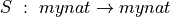 that returns the successor of its argument. (It’s an easy one-liner.) Now, instead of having to write mynat.succ n you can just write S n. Similarly define Z to be mynat.zero.
The binary functions on natural numbers include all of the operators familiar since first grade arithmetic: addition, subtraction, multiplication, division, exponentiation, and more. As an example, we will define a function that “adds” values of type mynat. We also demand that this function faithfully implement genuine natural number addition. So for example, we we add applied to S (S Z)) (representing 2) and S (S (S Z)) (representing 3) to return S (S (S (S (S Z)))) (representing 5).
The mystery that we address and resolve in this section is how to write functions that can deal with arbitrarily deeply nested terms. A value of type mynat can have any finite number of mynat.succ constructor applications in front of a mynat.zero, so we need to have a way to deal with such terms.
The resolution will be found in the concept of recursive function definitions. Let’s start with the addition function. We’ll call it add_mynat.
def add_mynat: mynat → mynat → mynat
| mynat.zero m := m
| (mynat.succ n') m :=
    mynat.succ (add_mynat n' m)

#reduce add_mynat zero three
#reduce add_mynat one three
#reduce add_mynat four three
As usual, we define the function by declaring its name and type, leaving out the colon-equals, and then giving rules for evaluating expressions in which the function is applied to two arguments. Each rule covers one case, where each case is an application of add_mynat to two arguments. The first rule matches on cases where the function is applied to mynat.zero and to any other value, m. Note that it is the matching construct itself that gives the name, m, to the second argument. In this case, the function simply returns m.
It’s the second rule where the “magic” happens. First, it matches on any first argument that is not mynat.zero. In this case, it must be an application of mynat.succ to a smaller value of type mynat. The matcher gives this value the name, n’. The second argument is, again, any natural namber, which is given the name, m. When such a case is encountered, the function returns the successor of the sum of n’ and m*.
For example, this rule causes the expression, add_mynat (S (S Z)) (S (S (S Z)))) to reduce to *S (add_mynat (S Z) (S (S (S Z))). The trick is that that inner expression is then reduced as well, and this process continues until no further evaluation is possible. Reduce that inner application yeilds the term *S (S (add_mynat Z (S (S (S Z))))). And now the first rule kicks in. The inner expression is simply reduced to (S (S (S Z))) and the whole expression is thus reduced to (S (S (S (S (S Z))))) as required.
That is how recursion works. But it’s not how you should think about recursion. The way to think about it is to see that the recursive definition is correct, and to trust it, without trying to unroll it as we’ve done here. You’ll agree that for any natural numbers, m and n, that (n + m) = S ((n-1) + m), right? It just makes sense. You don’t need to think about applying this rule n times to get a valid answer.
You’ll should also agree that if you repeatedly apply this rule to rewrite (n + m) as S ((n-1) + m, that eventually the first argument will reach zero, right? The unrolling can’t go on forever. Why, because, by definition, all terms of an inductive type are constructed by some finite number of applications of the available constructors. There can only be so many mynat.succ applications to mynat.zero in any mynat, no matter how large, and taking one away repeatedly will eventually get all the way down to nat.zero.
Therefore, we can conclude that (1) each unrolling step gives us a mathematically valid result, (2) if the unrolling eventuall yeilds an answer, it will be of type mynat, which is to say it will be some number of mynat.succ constructors applied to mynat.zero, and (3) the unrolling will always terminate in a finite number of steps. Specifically, it will always terminate in n steps, where n is the first argument to the function. We can also conclude that the time it will take to perform addition using this method is proportional to the value of n.
There’s an important insight to be had here. The addition of n to m is achieved by applying the successor function n times to m. At each step of the recursion, we strip one mynat.succ from n and put it outside the remaining sum of n’ to m. When there are no more mynat.succ applications to remove from n, we now have n applications of it to add_mynat mynat.zero m, which just evaluates to m. The result is n applications of mynat.succ to m. We thus define addition by the iteration of an increment (add one) operation.
We can now use this insight to see a way to implement multiplication. What does it mean to multiple n times m? Well, if n is 0, it means 0. That’s the base case. If n is not zero then it’s 1 + n’ for some one-smaller number, n’. In this case, n * m means (1 + n’) * m, which, by use of the distributive law for multiplication over addition, means m + (n’ * m). There’s the recursion. We see that n * m means m added to 0 n times.
EXERCISE: Define a function, mult_mynat that implements natural number multiplication.
EXERCISE: Define a function, exp_mynat that implements natural number exponentiation.
EXERCISE: Take this pattern one step further, to define a function that works by iterating the application of exponentiation. What function did you implement? How would you write it in regular math notation?
EXERCISE: Write a recursive function to compute the factorial of any given natural number, n. Recall that 0! = 1, and that for n > 0, n! = n * (n-1)!.
EXERCISE: Write a recursive function to compute the n’th Fibonacci number for any natural number, n. Recall that fib 0 = 0, fib 1 = 1, and for any n > 1, fib n = fib (n - 1) + fib (n - 2). How big must n be for your implementation to run noticably slowly? What’s the largest n for which you can compute fib n on your own computer in less than one minute of compute time? -/
4.8.3. Properties
We now prove that our implementation of arithmetic has key properties that it must have to be correct.
We’ll start with the claim that for any value, m, 0 + m = m. (We’ll just use ordinary arithmetic notation from now on, rather than typing out add_mynat and such).
The key to proving this simple universal generalization is to see that the very definition of add_mynat has a rule for evaluating expresions where the first (left) argument is mynat.zero. We can use this rule as an axiom that characterizes how our function works.
Lean provides a tactic called simp (short for simplify) that willsimplify expressions using the evealuation rules for any function definitions you specify. Here, then, is a formal, checked proof in Lean of our simple claim.
theorem zero_left_id:
    ∀ m : mynat,
        add_mynat mynat.zero m = m
:=
begin
intro m,
simp [add_mynat],
end
We just asked Lean to simplify the goal using the “simplification rules” specified by the two cases in the definition of add_mynat. Lean uses the first rule to reduce the sum of zero and m to m. The result is is m = m, which is proven true by automated application of the axiom stating that equality is reflexive.
Unfortunately, we don’t have such a simplification rule when the first argument is not zero, even if the second one is zero. So if we want to prove the proposition that for all n, n + 0 = n, we have no obvious way to do it. We need a new proof strategy.
This will again be proof by induction. But now we’re no longer in a situation where this proof technique is equivalent to simple case analysis for the constructors of an enumerated type.
Now, we’re in a situation in which arbitrarily large terms of a type can be built from smaller terms of the same type. Our mynat type thus has an infinite number of values, and there is thus no feasible way to prove a theorem by considering each value in turn.
Rather, we have to use an induction principle for our more complex type. The principle is no longer of a form that says, “if prove your proposition for each of n individual cases, you will have proved it for all cases”, because n is no longer finite.
What we encounter now is a new form of induction principle. What is says is that if you prove your proposition for your base case (here mynat.zero) and if you prove that if your proposition can be proved for any smaller value, n’ it can then be proved for a value constructed from n’, then you can conclude that it can be proved for all values.
Why does this make sense? Well, if a proposition is true for 0, and if whenever it’s true for any n’ then it’s true for n = S n’, then, in particular, it’s true for S 0, which is 1. And now that it’s true for 1, it must also be true for S 1, which is 2. And now because it’s true for 2 it must be true for 3. And so it goes, ad infinitum. It is therefore true for all values of our type.
The crucial element in this narrative is that there are two cases to prove. The base case is just a proof for a single element, but the case for the second constructor is an implication. If the proposition is true for some value, n’, then it’s true for a value constructed from n’. To prove this is to prove an implication. So we *assume the premise and then in that context we show that the conclusion follows. The premise is called an induction hypothesis. Case analysis using the cases tactic no longer works because it doesn’t introduce induction hypotheses into the context. The induction tactic does, and that makes all the difference.
Here’s an example. We prove that zero is a right identity for addition as implemented for mynat.
theorem zero_right_id :
    ∀ m : mynat, add_mynat m mynat.zero = m :=
begin
intro m,
-- proof by induction
induction m with m' h,
-- first the base case
apply rfl,
-- then the inductive case
simp [add_mynat],
assumption,
end
The proof is by induction. The with construct gives names, m’ and h, respectively, to (1) the smaller object from which m is assumed to have been constructed, (2) a proof for the assumption that the proposition is true for m’.
The base case is straightforward. The inductive case is where the action is.
Start by noticing and understanding m’ and h. Note that we can simplify the goal by applying the second rule once. Doing this effectively moves the mynat.succ to the outside of the sum. We then end up with a mynat.succ constructor application at front of the terms on both the left and the right of the goal.
The next action that the simp tactic takes is remove the mynat.succ function applications from the the front of the left and right sides of the equality. Such a move is not valid for any function, f. For example, if f returns zero no matter its argument, then f 10 = f 20 but 10 does not equal 20. The property of the constructors of an inductively defined type that makes this move valid is that they are injective.
If C is an any constructor and a1 and a2 are arguments, and if C a1 = C a2, then it must be that a1 = a2. It is the property of being injective that allows one to remove mynat.succ from the front of each side of the goal, which is what explains why the remaning goal is what it is after simp.
The result at this point is that the goal has been modified into one in which the induction hypothesis can be used to finish the proof. In this case, the remaining goal is exactly the hypothesis, h, so the proof is done.
The basic pattern that we see here is the one that occurs over and over in proofs by induction. First one must reformulate the goal using whatever facts one has on hand, with the aim of getting it into a form in which the induction hypothesis can be used. After that, some additional “algebra” will often be needed to completely finish it off the problem.
EXERCISE: Prove that our implementation of natural number addition has the property that adding n to one more than m yields one more than the sum of n and m. You will want to use induction.
lemma add_n_succ_m :
    ∀ n m : mynat,
        add_mynat n (mynat.succ m) =
        mynat.succ (add_mynat n m) :=
begin
_
end
EXERCISE: Give a paper an pencil proof, by induction, for the proposition that for all natural numbers, n, the sum of the numbers from 0 to n is n*(n+1)/2.
EXERCISE: A slightly different form of this proposition is that twice the sum of the numbers from 0 to n is n*(n+1). State and prove this proposition in Lean. By rewriting the claim, we avoid the need to use division, which complicates things.
There are many other properties that we would want to p prove about our own natural number arithmetic library to be completely and justifiably confident that it’s correct. Here we give one example: we state and prove the claim that (our implementation of) addition operation is commutative.
example :
    ∀ m n : mynat,
    add_mynat m n = add_mynat n m :=
begin
    intros m n,

    -- by induction on m
    induction m with m' h,

    --base case: m = zero
    simp [add_mynat],
    rw zero_right_id,

    -- inductive case:
    -- if true for m then true for succ m
    simp [add_mynat],
    rw add_n_succ_m,

    -- rewrite using induction hypothesis!
    rw h,

end
EXERCISE: State and prove the proposition that our implementation of addition is associative.
EXERCISE: State and prove the proposition that our implementation of multiplication is commutative and associative.
EXERCISE: State and prove the proposition that our implementations of addition and multiplication are such that multiplication distributes correctly over addition. That is, for all m, n, k, m * (n + k) = (m * n) + (m * k).
4.8.4. Lists (Sequences)
4.8.5. Data Type
We can import definitions from another file. Here we import our definitions from the mynat.lean file. The dot (.) tells Lean to look for that file in the same directory as this file.
import .mynat
Open the mynat namespace (in that file) so that we don’t have to prefix names with mynat.
open mynat
– Create a namespace for this file
namespace my_list_adt
We now introduce a type of “lists that contain objects of some other type, T.” For example, an object of type “my_list ℕ” would represent a list of value of type ℕ, while an object of type “my_list bool” would represent a list of values of type bool. Here’s the “inductive” declaration. Notice that, in constrast to nat and bool, this declaration has a parameter, T.
inductive my_list (T: Type) : Type
Now think about the type of my_list. Its type is Type → Type. We call my_list a type constructor or a polymorphic type. It takes a type as an argument and then returns a type, specialized for elements of the given type, as a result.
Generic types in Java and template types in C++ similarly take type parameters and yield new types specialized for handling of values of the specified argument type.
Now we give the constructors for our polymorphic type. The first one, my_nil, is a constant term of type (my_list T). We will interpret it as representing the “empty list of values of type T.”“
| nil: my_list
And here’s the interesting part. We now provide my_cons as a constructor used to produce a bigger list from a given list by tacking a new value onto its front.
The constructor takes a value, h (short for “head”), of type T, the value to be tacked on; and then it takes a value, t (short for tail), the smaller list onto which h will be tacked. The result is a new my_list, represented by the term, (my_cons h t), which we interpret as the list starting with h as the value at its head, and with the whole smaller list, t, as its tail (the rest of the list).
| cons: T → my_list → my_list

open my_list
4.8.5.1. Examples
- list of mynat
- list of ℕ
- list of bool
-- some lists of mynat values

def empty_mynat_list : my_list mynat :=
    (nil mynat) -- []

#reduce empty_mynat_list

def zero_mynat_list :=
    (cons zero empty_mynat_list) -- [0]

#reduce zero_mynat_list

def one_mynat_list :=
    (cons one zero_mynat_list) -- [1,0]

#reduce one_mynat_list

def two_mynat_list :=
    (cons two one_mynat_list) -- [2,1,0]

-- A list of ℕ values! [2,1,0]

def two_nat_list :=
    (cons 2
    (cons 1
    (cons 0
    (nil ℕ))))

#reduce two_nat_list


-- A list of bool values [tt,ff,tt]

def a_bool_list :=
    (cons tt
    (cons ff
    (cons tt
    (nil bool))))
4.8.6. Functions
/-
Adding functions to our algebra
-/

-- If list is empty return true else false
def isNil { T : Type } (l : my_list T) : bool :=
match l with
| (nil T) := tt
| _ := ff
end

#reduce isNil a_bool_list
#reduce isNil empty_mynat_list
Note that T is an implicit parameter here. Lean can infer T from l.
-- Length of l. A recursive function.
def length : ∀ { T : Type }, my_list T → ℕ
| _ (nil T) := 0
| _ (cons h t) := 1 + (length t)
In the pattern matches here, Lean requires that we match on both arguments, but we do not want to give a new name to T, so we use _ as a wildcard. We can then use the T that is declared on the first line as a value in the pattern for the nil list.
#reduce length empty_mynat_list

-- Append two lists

def append :
    ∀ { T : Type },
        my_list T → my_list T → my_list T
| _ (nil T) l2 := l2
| _ (cons h t) l2 := cons h (append t l2)


#reduce a_bool_list
#reduce append a_bool_list a_bool_list
4.8.7. Properties
-- Here's one, no induction needed
theorem nil_append_left_zero :
    ∀ { T : Type },
    ∀ l2 : my_list T,
    append (nil T) l2 = l2 :=
begin
intro T,
intro l2,
-- simplify using rules for append
simp [append],
end
– But this requires induction
theorem nil_append_right_zero :
    ∀ { T : Type },
    ∀ l1 : my_list T,
    append l1 (nil T) = l1
:=
begin
intro T,
intro l1,
induction l1,

-- base case
simp [append],

-- inductive case
simp [append],
assumption,
end
– A desired property of append!
theorem append_length :
    ∀ { T : Type },
    ∀ l1 l2 : my_list T,
    length (append l1 l2) =
    (length l1) + (length l2) :=
begin
intros T l1 l2,
--cases l1 with h l1' --no work!
induction l1 with h l1 ih, -- need ih

/-
base case: simplify using
definitions of length, append
-/
simp [append, length],

-- inductive case

-- simplify goal as usual
simp [append, length],

-- critical: rewrite using ih!!!
rw ih,


/-
See if Lean can figure out to
figure out to apply commutativity
of addition.
-/
simp,

-- yay, qed!
end

end my_list_adt
4.9. Binary Trees
4.9.1. Data Type
We define a polymorphic type, “tree”, just like tree_nat, but where the value stored in a node can be of any type, T. Then define aTree’ to be the same as aTree except that it’s now of type tree rather than of type tree_nat. Make the type argument implicit. Finally define a tree of strings, aTree’‘, just like aTree’ except that 3 is replaced by “Hi!” and 2 is replaced by “Jo”.
inductive tree { T : Type } : Type
| empty : tree
| node : T → tree → tree → tree
Given this type definition, we can now construct binary trees with values of any types. Here are three examples.
The first is an empty tree of natural numbers. The second is a non-empty tree of natural numbers. The third is a non-empty tree of strings. We start by defining an empty tree of natural numbers. We repeat the definition of the tree data type so that you can try this example in your browser.
inductive tree { T : Type } : Type
| empty : tree
| node : T → tree → tree → tree

def anEmptyTreeOfNats := @tree.empty nat
The only potential mystery in this example is the use of @ to turn off implicit arguments. Because the empty tree constructor takes no arguments, Lean has no way to infer the type parameter, T, so we must give the type argument explicitly. The @ symbol tells Lean not to try to infer T automatically, but to allow us to give it explicitly. We use @ whenever implicit arguments are specified but where we need to turn off this behavior so that we can give a type argument explicitly. We need to do that in this case because otherwise Lean doesn’t have enough information to infer the value of the type parameter, T.
Here are our second two examples. We again repeat the type definition to make this example self-contained. Take note of how we lay out the code, with a tree constructor on one line and each of its arguments indented on the following lines. We find that laying out definitions of recursive values in this way makes them easier to write and to read.
inductive tree { T : Type } : Type
| empty : tree
| node : T → tree → tree → tree

def aNatTree : tree :=
    tree.node
        3
        (tree.empty)
        (tree.node
            2
            tree.empty
            tree.empty)

def aStringTree : tree :=
            tree.node
                "Hi!"
                (tree.empty)
                (tree.node
                    "Jo"
                    tree.empty
                    tree.empty)
4.9.2. Functions
Given our polymorphic tree data type, we can now write functions that operate on trees. Here are several examples.
Our first function, which is not recursive, illustates the use of pattern matching to determine whether a given tree is empty or not. It returns true or false, respectively, in these cases. The second example illustrates the use of recursion to count the number of nodes in a given tree.
inductive tree { T : Type } : Type
| empty : tree
| node : T → tree → tree → tree

/-
The number of nodes in an empty tree is zero,
while the number of nodes in a non-empty
tree is one (for the "top" node) plus the
number of nodes in each of the subtrees.
-/

def num_nodes : ∀ {T : Type}, @tree T → nat
| T tree.empty := 0
| T (tree.node t c1 c2) :=
    1 + num_nodes c1 + num_nodes c2

/-
We now prove a property about our function. What we
prove is that the size of any non-empty tree is one
more than the sizes of its two sub-trees. Please refer
to the following commentary for an explanation of the
proof.
-/
example :
    ∀ {T : Type} (b1 b2 : @tree T) (t : T),
    @num_nodes T (@tree.node T t b1 b2) =
    1 + @num_nodes T b1 + @num_nodes T b2 :=
begin
intros T b1 b2 t,
induction b1 with t' b1' b2' Ih1 Ih2,
simp [num_nodes],
simp [num_nodes],
end
4.9.3. Properties
The proof of the conjecture claiming that the size of any non-empty tree is one more than the sum of the sizes of its two children is by induction. But it’s a very simple case of proof by induction that could have been handled by simple case analysis instead (like induction but without the need for any induction hypotheses). Nevertheless, it’s instructive to see and understand the elements of the proof states as one goes through this proof.
The first thing to understand is the induction principle for the tree data type. In general, and induction principle says that (1) if the base cases of a type have some property, and (2) if whenever some smaller values of the type have it, any one-larger value built by applying any constructor to those smaller values also has the property, then (3) all values of the type have that property.
What we see that’s a bit new in this case is a situation where a one-larger value of type tree is being built from two smaller values of the same type. The induction principle thus says, informally, that if (the base value, tree.empty, has the property), then (if whenever a smaller tree, b1’, has the property and a second smaller tree, b2’, also has the property, then a one-larger tree *tree.node t b1 b2 also has the property), then all trees have the property. The key aspect to take note of is that in the inductive case there are now two induction hypotheses: b1 has the property and b2 has it, too.
Let’s look in more detail at each of the two cases, starting with the base case. In this case, b1’ is the empty tree, and we therefore must show that num_nodes (tree.node t tree.empty b2 = 1 + num_nodes tree.empty + num_nodes b2. Note that tree.empty is substituted for b1’ because that is the case we are looking at: where b1’ is the empty tree. The first case in the definition of num_nodes tells us exacty how to simplify this expression, so that the goal follows from the reflexivity of equality.
Now let’s look at the recursive case. The proof state is a bit busy, but that makes it even more important to read and understand it. Start with the context. Let’s take it step by step. The first line is the assumption that T is a type. Second, we’ve assumed that b2 is an arbitrary tree. Third, we’ve assumed that t and t’ are values of type T, i.e., values that can be incoporated into tree nodes. Fourth, we’ve assumed that b1’ and b2’ are two smaller trees. The fifth and sixth lines are the induction hypotheses that come from Lean having applied arrow introduction for us on the way to our proving the inductive case. The first induction hypothesis is that if we build a bigger tree from t, b1’ and b2, then the property of interest holds; and the second induction hypothesis says the same thing for b2’. In other words, we’ve assumed that the sizes of trees built directly from b1’ or b2’ are each one more than the sizes of their two subtrees.
In this context, what we now have to prove is that if we build a one-larger tree from b1 and b2, where b1 is itself now a non-empty tree built from b1’ and b2’, both of which we have assumed have the property we care about, then the resulting tree will also have that property: that the size of this tree is one more than the sizes of b1, which is now expressed as tree.node t’ b1’ b2, and b2.
The proof of this is again by mere simplification of the expression to be proved. Just apply the rule for computing the size of a non-empty tree to the left side of the equality to be proved. The result is exactly the expression on the right side, and Lean then finishes the proof by applying the principle of reflexive equality. In more complex proofs by induction, one will have to apply one or both induction hypotheses to prove the goal.
EXERCISE: Show formally that you not need to use induction to construct a proof of the preceding conjecture; that case analysis (without the need for induction hypotheses) suffices.
4.10. Certified ADTs (Optional)
In mathematics, logic, and computer science, we care not only about the set of values of a given type, and about the functions that can be applied to such values, but also about key properties of these things. For example, in natural number arithmetic, we care about: (1) the values of the natural number type (0, 1, 2, …); (2) functions that can be applied to values of this type (negation, addition, etc); and (3) properties of these functions (e.g., addition is associative and commutative, that multiplication distributes over addition, etc).
Indeed, the fundamental building block of practical modern software systems combines these three elements: a data type, a set of functions that operate on values of this type, and a set of propositions concerning properties of these values with functions with proofs. We will call such a building block a certified abstract data type (CADT). It is an abstract data type in the sense that it combines a data type and a set of functions that operate on values of the type. It is certified in that there are proofs of propositions concerning properties of values of the type and of functions that operate on such values.
Classes in many object-oriented languages can be thought of as defining abstract data types. The data members (or fields) of a class specify the possible data values of the type. The member functions specify functions that operate on values of the type. In object-oriented programming, such a function, $f$, generally takes as its first argument an object, m, of the given type, with notation m.f(…). You can think of m here as just the first argument to the function, f.
There’s a bit more to object-oriented programming (OOP) than just this simple idea. In particular, in OOP languages, the function, $f$, that gets invoked generally depends not only on the type, but also on the sub-type of m. This mechanism is called dynamic dispatching, or dynamic polymorphism. We do not discuss it any further in this course.
As for propositions and proofs, ordinary programming languages lack the expressiveness to represent them, and so they remain unstated and unproven in most cases in practice. An important use case for constructive logic proof assistants to support the development of certified ADTs and certified systems from such certified building blocks. Development methods of this kind are increasingly important in the production of provably secure and other critical systems: for finance, ecommerce, defense, critical infrastructure systems (such as transportation), etc.