3. Proofs
3.1. Introduction
The preceding section of these notes introduced the language of predicate and constructive logic, but it left hanging the question of how to:
- construct proofs that you need
- extract information from proofs you already have
This section of the book answers these questions by teaching you how to construct and use proofs.
3.1.1. How to Design Proofs
In constructive logic, propositions are types and proofs are programs. To design a proof is thus akin to designing a program. Each such program is nothing but an application of a proof-constructing function, a.k.a, an inference rule, to arguments of the right types. Often, these arguments will include other proofs. The problem of designing a proof thus breaks into two sub-tasks.
3.1.1.1. The Problem to be Solved
Suppose you want to construct a proof, p, of some proposition, P. As you recall, P, a proposition, is also a type in constructive logic, so you can view your task as nothing other than constructing a term of type P. Such a term will always be in a specific form. It will always be a function application term, f a b c …, where f is a proof-building function (an inference rule); where a, b, c, etc., are values of the types f requires as its arguments; and where f when applied to such values returns a value, a proof, of the right type, namely a proof of P.
3.1.1.2. Step 0: Understand What Type of Proof is Required
3.1.1.3. Step 1: Select an Inference Rule
The first step is to select an inference rule, a proof-building function, to use to construct the proof you seek. You are highly constrained in your choice, because you must select an inference rule that constructs a proof of the required type. For example, if you require a proof of a proposition, a = b, then you have no choice but to select an inference rule that returns a value of this type: a proof of this proposition.
3.1.1.4. Step 2: Apply It to Arguments of the Right Types
Step 2: Having selected an inference rule to use to construct a proof of a given proposition (your goal), the second step is to apply the function to arguments of the right types. Often the arguments that are required are themselves proofs of other propositions. Having selected a rule to apply the problem is reduced to zero or more sub-problems: to construct arguments of the right types to which the selected inference rule can be applied to construct the final proof value.
3.1.1.5. Method: Top-Down, Type-Guided Refinement with Backtracking
The challenge, of course, is that it’s not always easy to come up with values of all the argument types required to apply an inference rule. This is true especially when an inference rule takes as arguments other proofs that you do not already have on hand. In this case, developing these smaller proofs, or lemmas, becomes the main challenge.
The crucial idea at this point is that you can give a complete proof, in the form of an application of the top-level inference rule, but leave holes in it where these arguments are required. Lean will then present them to you as sub-goals. And, now for the trick: You solve them in the same manner, by the recursive application of the same top-down, type-guided refinement technique.
If you get completely stuck, then you have discovered that perhaps you went do the wrong path, and you have to backtrack and try something else. So the overall approach is top-down, type-guided refinement with backtracking. That is how to design proofs.
3.1.1.6. Discussion
To start with, we have only the basic inference rules of natural deduction. These are the assembly language of proof construction. As we go along and prove richer and richer theorems, the proofs of those theorems, checked for logical validity by Lean, become higher-level inference rules that you can use later on to avoid re-doing a lot of low-level work.
Learning the set of basic inference rules and how you can compose them into larger proof-building functions to prove more interesting propositions is the essential aim of this chapter. As we go, we will develops a library of richer rules/functions/proofs. You will want to remember what proof-building rules we have at hand, including both the basic rules of natural deduction and the higher-level rules that we implement ourselves. Understanding these concepts is the main intellectual challenge in this section of the course.
To succeed, you must know the basic inference rules of natural deduction. You must be fluent enough in being able to recall and use to implement new proof-building functions to prove more complex and interesting propositions.
3.1.1.7. Introduction and Elimination Rules
The rules for using and constructing proofs, in ways that are logically valid, are known as elimination and introduction rules, respectively. The introduction and elimination rules together are known as the inference rules of a logic. Introduction rules are used to construct proofs of a particular form (using a particular connective or quantifier), while elimination rules are used to de-construct proofs of a particular form to obtain information contained within them. The inference rules that we will meet in this section of the notes are the fundamental rules for logically valid reasoning in the system of reasoning generally known as natural deduction. Natural deduction was invented long before automated proof assistants such as Lean were built. It is the framework on which such automated reasoning tools are based.
3.1.2. Structure of Each Following Chapter
The central idea on which this section of the course is organized is that each syntactic form of proposition has its own corresponding introduction and elimination rules. This section thus has one chapter for each form of proposition. Each of the following chapters is organized in the same way. It first reviews the form of proposition that is the subject of the chapter, and its intended meaning. The heart of each chapter presents the corresponding introduction and elimination rules and how these rules enforce the intended meanings of the connective or quantifier being considered. Each inference rule is presented in a textual form, using what we will just call inference rule notation. Then at the core of each chapter is a presentation of each inference rule as a function in Lean. We introduce additional related concepts in the context of these chapters. Each chapter wraps up with an explanation of how one would write informal proofs using the given inference rules.
Whether one is using Lean or not, these are the principles of logical reasoning by which one constructs and uses proofs of propositions. To learn proofs requires fluency with these rules. The aim of this section of the course is to develop fluency, not just a superficial understanding of, but the ability to apply, these rules.
3.1.3. Inference Rules are Functions in Constructive Logic
In constructive logic, inference rules are formalized as functions. They are define in just the right ways to enforce the intended interpretations of corresponding forms of propositions. Introduction rules (functions), for constructing proofs, generally takes arguments of certain types, often proofs of other “smaller” propositions, as arguments, enforcing the constraint that certain things must be true (and there are proofs) before proofs of “bigger” propositions can be formed. Similarly, elimination rules take proofs as arguments and can only extract and return certain values from them. The Lean type checker is the enforcer of logical consistency!
For example, the introduction rule (function) for constructing a proof of  , requires that proofs of
  and of
  be given as arguments. The type checker will reject proof values that are not of the required types, e.g., and . The upshot is that it’s not possible to construct a proof of in Lean unless one already has individual proofs of and of . A proof of a conjunction thus guarantees that proofs exist for each conjunct, enforcing the meaning of the and connective.
Similarly, from a given proof of , one can apply elimination rules (functions) to obtain individual proofs of and . These are the return types of the two elimination rules for conjunctions. In general it is not possible to derive a proof of some other proposition, say  , from no more than a proof of
  as there is no rule available for doing this.
In traditional paper-and-pencil discrete math courses, there is often a strong emphasis on learning what are called proof strategies. For example, proof by negation is a strategy for proving negations: propositions of the form not P. It works by assuming that P is true, showing that that leads to a contradiction, and then concluding from that that P must be false (i.e., that not P is true). We will discuss these so-called proof strategies in this chapter. What you will see, however, is that what they really amount to is nothing other than the application of certain inference rules, often with the result of transforming a current proof goal (a proposition to be proved) into a different form, in a valid way, taking you one step closer to having a complete proof.
3.1.4. Aims of this Section of the Course
In a nutshell, then, for each of the syntactic forms of proposition, there is an associated set of proof construction (introduction) and information extraction (elimination) rules. Proof strategies are just inference rules. The overarching objective of this section of the course is to have you deeply understand, remember, and be able to apply all of these rules. You will often need to apply combinations of rules/functions, to construct proofs. You will come to feel that constructing proofs is very much like (and it is!) constructing programs: ones that take arguments of certain kinds, including proofs, and that return values of other kinds, including proofs. Whether you are doing informal proofs on paper and pencil or using Lean or another proof assistant, you will use these rules of reasoning. All of mathematics, logic, and computer science depend on them. You should make mastery of these rules your learning goal for this section of the course.
Inference rules are functions, and proofs are obtained by applying such functions to the right kinds of arguments. Constructing proofs of propositions turns out to be a programming problem! One must produce a program that constructs a proof of a proposition to be proved. A proof is a value logical type, of the proposition, that is the return type of the function.
The remainder of this chapter starts with proofs of equality propositions, then moves on to universal generalizations; false and true; conjunctions; implications; bi-implications (equivalences); disjunctions; negations; and finally existentially quantified propositions.
3.2. Equality
In mathematical and logical reasoning, we often need to express the proposition that two terms are equal, or not. For example, in specifying how an online system should work, we might want to state that if s and t are terms that represent the same Person, then the account numbers associated with s and t must be the same. We could write this in logic with an expression something like this:  . In this chapter, we present the concept of equality precisely as it is formalized in typed predicate and constructive logic.
There are two basic issues to understand. The first is how to use what Lean calls the eq predicate, which takes two (explicit) arguments, such as s and t, to form propositions of the form, s = t. The second issue is to understand the inference rules available to construct and use proofs of such propositions.
3.2.1. Formula
In a typed predicate logic, equality is a predicate. In Lean, the predicate is called eq. This predicate takes three arguments: a type, T, and two terms, s and t of type T (for whatever type might have been given for the argument T). Lean infers the value of T from the arguments s and t, and so is never given as an explicit argument. To form a proposition using eq, one thus just applies it to two arguments, which must be of the same type. The result of the #check command confirms that anEqualityProposition is a proposition.
Here’s an example. We assign to anEqualityProposition the proposition, 1 = 1. In this case, Lean infers that the value of the type argument, T, is nat. The #check command confirms that anEqualityProposition is a proposition. On the other hand, trying to form the proposition that 1 = tt doesn’t work at all, because the two terms are not of the same type.
def anEqualityProposition := eq 1 1
#check anEqualityProposition
def noCanDo := eq 1 tt
For each and every type, T, the eq predicate can thus be used to form propositions of the form eq s t, which can also be written as s = t. The expression s = t is defined to be a notation that means exactly eq s t. Here’s a formal statement of this proposition, along with a proof of it, constructed incrementally using a Lean tactic script, starting and ending with the keywords, begin and end, respectively. We will cover proof scripts in increasing depth and detail in this section of these notes.
example: ∀ T: Type, ∀ a b: T, (eq a b) = (a = b) :=
begin
  intros,
  exact rfl
end
Many functions and predicates defined in Lean’s libraries, which are automatically imported when we use Lean, have convenient notations. For example, the term 1 + 2 is just a nice notation for nat.add 1 2, where nat.add is the name of the function defined in Lean’s libraries for computing sums of natural numbers.
Here are a few examples where we form equality propositions using the = notation rather than eq. These examples also show that we can form equality propositions for objects of arbitrary types, as long as the objects on the two sides of the = sign are of the same type. (A kind of exception is that if Lean knows of a way to a value of one type into a value of another type, then you can write equalities involving both types and Lean will do the coercion for you.) The last line of this code block is an example where Lean issues a type error, which expresses that Lean found no way to covert the Boolean value, tt into a value of type nat.
#check eq 0 0   -- a proposition
#check 0 = 0    -- same, nicer notation
#check 1 = 1    -- another proposition
#check 0 = 1    -- a third proposition
#check tt = ff  -- involving booleans
#check "Hi" = "H" ++ "i"    -- strings
#check 1 = tt
3.2.2. Interpretation
What we want a proposition, s = t, to mean is that the two terms reduce to the same values. In the second to the last example above, for instance, we want it to be the case that "Hi" is treated as being equal to (the string denoted by the the function application expression) "H" ++ "i", because they mean the same string.
Whether values are written directly or indirectly by the application of functions to arguments, if they are the same value, then we want it to be true, which means that we want to be able to construct a proof, that s = t. In any other where s and t do not represent exactly the same value, we want it to be impossible to construct such a proof. It is the provisioning of specific introduction (proof construction) and elimination (proof utilization) rules that enforces this, our intended, interpretation of equality propositions. We now turn to these inference rules, starting with the single introduction rule, which you can now think of as a function for producing proofs of equality propositions.
3.2.3. Introduction
We previously mentioned that introduction rules are used to introduce or construct proofs of a particular type. The natural deduction reasoning system provides us with one such inference rule for constructing proofs of equalities: eq.refl. The eq.refl rule is used to construct or introduce a proof that two objects are equal.
Let’s unpack the name of this rule/function. This name has two parts, eq and refl. In this context, eq is a namespace associated with the eq predicate, and refl is the name of the proof-building function, defined within this namespace. To use the function from outside the namespace, one must either open the eq namespace, which we will not do, or use the qualified name, eq.refl.
3.2.3.1. Proving t = t
This inference rule, a function, takes two arguments: a type, T, and a single value, t, of type, T. It then constructs and returns a proof of t = t. In natural deduction, and so in Lean, this is the only way to construct proofs of an equality. Here’s an example in which we assert that the proposition, 1 = 1, is true, by asserting that we can bind a proof to an identifier, one_eq_one, of this type (remember, propositions are types), and then showing that we can do this by using eq.refl to construct a proof of (a value of type) 1 = 1. The #check command confirms that one_eq_one really is now bound to a value (namely eq.refl 1) of type (a proof of) 1 = 1.
def one_eq_one : 1 = 1 := (eq.refl 1)
#check one_eq_one
EXERCISE: Explain why you could never use eq.refl to construct a proof that that two different values are equal.
3.2.3.2. Proving s = t (different terms for same value)
So, how does this work when applied to an equality proposition with two different terms that nevertheless mean the same thing? Consider the terms, s := 2 and t := 1 + 1. The trick to understand that if one writes s = t, then Lean evaluates s and t before producing the proposition against which a proof is type checked. So if s and t reduce to the same value, then it will be possible to prove s = t, using either eq.refl s or eq.refl t as a proof.
#check eq 2 (1 + 1)
#reduce eq 2 (1 + 1)
3.2.3.3. Inference rule notation
In logical writing, and also in such computer science fields as programming languages and software verification, inference rules, which are really just functions, are presented in a stylized form. Here is the eq.refl presented in this textual inference rule style. What is says is that if you apply eq.refl to a value, t, of some type, T, where the curly braces signal that type inference will be used to infer the value of T (from t), then the return value will be of type eq t t. That is, it will be a proof of t = t.

Here are a few more examples.
def z_eq_z : 0 = 0 := eq.refl 0
def z_eq_z' : 0 = 1 - 1 := eq.refl 0
def z_eq_z'' : 0 = 1 - 1 := eq.refl (1 -1)
def ff_eq_ff : ff = band ff tt := eq.refl ff   -- boolean and
def hi_eq_hi : "Hi" = "H" ++ "i" := eq.refl "Hi"
3.2.3.4. Using rfl as a shorthand
In many cases, Lean can infer not only T, but even the value t, from context, namely from the type of proof that is to be produced. A version of the eq.refl rule that works this way is called rfl. It’s easier to type and to read than eq.refl t, and so is preferred when it works. Here are the preceding examples using rfl.
def z_eq_z : 0 = 0 := rfl
def z_eq_z' : 0 = 1 - 1 := rfl
def z_eq_z'' : 0 = 1 - 1 := rfl
def ff_eq_ff : ff = band ff tt := rfl
def hi_eq_hi : "Hi" = "H" ++ "i" := rfl
EXERCISE: Explain precisely why eq.refl (or rfl) can never be used to derive a proof of 0 = 1.
3.2.3.5. Inference rules are functions
As show now be clear, inference rules in natural deduction, and thus in Lean, act like, and literally are, functions. You must provide arguments of the right types, and in return they produce values, here proofs, of desired kinds: in this case, proofs of equalities.
In many cases, inference rules will require not only types and computational values as arguments, but also proofs of previously proved or axiomatically accepted propositions. As we discussed above, for example, the introduction rule for constructing a proof of a conjunction requires proofs of the two conjuncts as arguments. Because Lean is strongly and statically type-checked, it will not permit the application of an inference rule unless valid value, including such proofs, are given for all arguments. In this way Lean enforces the consistency, the correctness, of logical arguments, formulated as proofs. So, you can now think of eq.refl in two different ways: as a logical inference rule, and as a proof-constructing function.
3.2.3.6. Top-Down, Type-Driven Refinement
We’ve now seen that we can prove a proposition by giving an exact proof term. Here we prove the proposition, 0 = 0, by giving an exact proof term (a value of a propositionall type).
lemma zeqz : 0 = 0 := eq.refl 0Just as functions definitions in ordinary programming can be pretty complex, proof terms can be, too. They can be so complex that they are very difficult to just write out all at once. Of course this is true of ordinary functions as well.
A fundamental approach to dealing with the complexity of definitions that we need to produce is to use abstraction. Abstraction is selective emphasis on the most important details of a solution, leaving holes where certain details will be filled in later. They key is to be sure that the overall solution structure works, and that it will lead to a good solution as long as those holes can be filled in with appropriate details later. One then proceeds to use the same approach to fill in each hole.
In Lean, the type of value needed in a given context is always known. The type of an overall proof term is just the type defined by the proposition to be proven (e.g., 0 = 0). We know that there’s only one type of proof that will do here. It’s the application of the eq.refl inference rule to some value. That some value is a hole! And holes have types. In this case, the definition of eq.refl requires that the hole be filled with a value of type, nat. Lean infers that from type of the values (the zeros) in the proposition. One can now proceed to work to achieve the sub-goal of filling that hole with a term of the right type. In this case, it’s a term of type, nat, and in particular what’s needed is the value 0.
it’s hard to write an exact proof term (here,
eq.refl 0). In these cases it can help to figure out a proof term step by step, in a type-drive, top-down, structured approach. Lean supports such stepwise development of proof terms. One can include underscores in proof terms as tactic-based proving. Here’s an equivalent tactic-based proof.In Lean, this approach to using top-down, type-driven refinement to develop proofs, or even ordinary functions or other values, can be done in at least two ways. One way to do it is to write out proof terms using underscore characters for the holes. Lean will show each one as a goal that remains to be achieved before the overall term is finished. Another equivalent way is to use tactic scripts to construct proofs. Let’s see that now.
First, with incomplete proof terms.
example : 0 = 0 := _
Now with a tactic script.
example : 0 = 0 :=
begin
end
Now open the Lean Messages panel (if it’s not already open) by typing control-shift-enter or command-shift-enter (Windows/Mac). Now place your cursor first at the start of the “exact”. The message window will display the “tactic state” at this point in the script. The state say that nothing is assumed and the remaining goal to be proved is 0 = 0. Now move your cursor to the next line, before the end. The tactic state is empty, nothing is left to be proved, QED.
Define zeqz’’ as also being of type0 = 0, but after the:=, just write begin on the next line and then an end on the following line. You need to type the begin and end lines before continuing. Put a new line between the begin and end lines, and then insertapply ex.refl,(do not enter0) and see what happens. In Lean you can “apply” inference rules with incomplete information. Sometimes Lean will complete the proof with information it can infer, but often it will change the proof state to a new state requiring you to prove additional information. This approach is useful when a single inference rule will not complete the proof.
3.2.4. Elimination
Whereas introduction rules give us ways to construct proofs that we need, elimination rules give us ways to use proofs that we already have. As we previously mentioned, elimination rules are used to extract information from proofs of a particular type, so an equality elimination rule will be used to extract information from a proof that two objects are equal.
Suppose we have a proof of some proposition involving s, and we also have a proof of s = t. To be concrete, suppose we have a proof of Kevin is from Charlottesville and we also have a proof of Kevin = Tom, maybe because Kevin uses Tom as an alias. Then we should be able to take advantage of (use) the proof that Kevin = Tom to convert the proof that Kevin is from Charlottesville into a proof that Tom is from Charlottesville.
This concept is formalized by the inference rules that in Lean is called eq.subst. Here is the rule itself, presented in inference rule style.

This rule takes six arguments, the first four of which are inferred. When applying the rule one gives only the last two arguments explicitly. The first four arguments are a type, T; a predicate, P, on values of type, T ( ); and two values, a and b of type T. The last two arguments (from which the preceding four are inferred), are, first, a proof of the proposition, a = b, and second, a proof of the proposition, P a. The latter is the proposition that a has the property represented by the predicate, P. What the rule returns is a proof of the proposition, P b, that b also has this property.
Here’s an example in which we formalize the informal argument about Kevin and Tom above.
axioms (Person : Type) (Kevin Tom : Person)
axiom kevinIsTom : Kevin = Tom
axiom isFromCville: Person → Prop
axiom kevinIsFromCville: isFromCville Kevin
example : isFromCville Tom :=
eq.subst kevinIsTom kevinIsFromCville
You can see that eq.subst is an elimination rule for eq propositions because it requires one to provide, to already have, a proof of a = b as an argument. This proof is then used, along with the additional proof of P a, to construct and return a proof of P b.
3.2.5. Properties
From the basic introduction and elimination rules for equality, one can deduce that the equality relation has several additional important properties. In particular, equality is reflexive, symmetric, and transitive, making it also what we call an equivalence relation.
3.2.5.1. Reflexivity
A relation in which everything is related to itself is said to be reflexive. Equality is reflexive in the sense that, for any value, a, of any type, T, we can obtain a proof of a = a. Every object is equal to itself. We can always construct a proof of a = a no matter what a is. To do this, we use eq.refl, or its shorthand form, rfl.
3.2.5.2. Symmetry
A relation in which if a is related to b then b is also related to a is said to be symmetric. Equality is symmetric in the sense that for any two objects, a and b, if a = b then b = a. What this means in Lean is that if we’re given a proof of a = b, we can apply a rule, not surprisingly called eq.symm, to obtain a proof of b = a.

Let’s see it in action in five lines of code.
def a := 1
def b := 2 - 1
lemma ab : a = b := rfl
#check ab           -- a proof of a = b
#check (eq.symm ab) -- a proof of b = a!
What we see is that eq.symm is really just another function that performs this logical inference automatically for us.
3.2.5.3. Transitivity
Finally, a relation is said to be transitive if a = b, and if b = c, then a = c.
Here’s an example in Lean.
axiom T : Type
axioms (a b c : T) (ab : a = b) (bc : b = c)
example : a = c := eq.trans ab bc
3.2.5.4. Equivalence
A relation, such as eq, that is symmetric, reflexive, and transitive is said to be an equivalence relation. We will discuss equivalence relations in more detail later in this course.
For now it suffices to observe that equality is an equivalence relation on terms. Terms that reduce to the same value are equivalent under Lean’s definition of equality, even if they are not expressed in exactly the same form. So, for example, 2 is equivalent to 1 + 1, to 4 - 2 and to an infinity of other terms under the equality relation.
An equivalence relation divides up the world into sets of values that are all equivalent to each other. We call such sets equivalence classes. Equivalence classes are disjoint in the sense that objects in one equivalence class are never equivalent to objects in a different equivalence class.
EXERCISE: Explain why equivalence classes must be disjoint.
3.2.6. Proof Irrelevance
An interesting case of equivalence is at the heart of Lean. In general, there are many ways to prove a given lemma or theorem. Each proof is nevertheless of the type of the proposition that it proves, and each suffices as evidence to justify a truth judgment for the proposition. In cases where one’s aim is simply to prove a proposition, the particular proof object that is used doesn’t matter. We say that the particular proof is “irrelevant.”
In Lean, different proof terms for the same proposition type are considered to be equal. So all proofs of a given proposition are equivalent (equal) in this sense, even if they are expressed in different ways.
EXERCISE: Demonstrate that different proofs of the same proposition are equivalent with an example.
3.2.7. Formalization (Optional)
In Lean, you can use the #print command to see the definition of any term. Let’s see how eq is defined.
#print eq
Consider the first first line: inductive eq : Π {α : Sort u}, α → α → Prop. The inductive keyword indicates that a new type, or in this case a way of creating new types, a family of types, is being defined. The funny Pi symbol can be read as saying “for any”, so Π {α : Sort u} can be read as saying, “for any Sort,  , whether Sort 0 (Prop), Sort 1 (Type), etc. The whole first line then says that eq is a kind of function that takes what we can refer to simply as some type, , and two values of this type, and that returns a proposition, which is itself a type. The curly braces indicate that the type is inferred from the other arguments. For example, the term eq 1 2 can now be seen as being (reducing to) a proposition, written simply as eq 1 2 or as 1 = 2.
Now we wish to enforce an interpretation of such proposition as asserting that the two values are equal. So we want there to be a proof of such a proposition if and only if the next two arguments are equal, at least when reduced. To this end, the definition of eq provides a means, a constructor, for building proofs of such propositions. It is called eq.refl. It takes one argument, a, of type , where is inferred from a. It then returns a value of type a = a, which is of type, i.e., that is a proof of, that proposition, eq a a. This constructor is the one and only introduction inference rule for equality. Because there are no other constructors for values of this eq type, nothing can be proved equal to itself that isn’t equal to itself! In this way, we use the definitions of inference rules to enforce our desired interpretations of given forms of propositions, here propositions that assert equalities between terms.
3.2.8. Natural Language
Natural language proofs involving easy equalities are usually written very concisely. A proof of t = t would usually be written as something like this: “It’s trivially the case that t = t.”
In fact, you can write a proof like this in Lean using a proof tactic. A tactic in Lean is a program that looks at what information you have that can be used (called a context) and what is to be proved (called a goal), and, based on its programming, tries to help you toward having a proof. Tactics thus automate certain aspects of proof construction.
axioms (T : Type) (a : T)
example : a = a := by trivial
3.2.9. Exercises
- First, write a textual inference rule, let’s call it eq_snart. It says that if T is any type; if a, b, and c are values of this type T; and if you are given proofs of a = b and c = b (notice this is not b = c), then you can derive a proof of a = c.
- Now “prove” that this rule is valid by implementing it as a function that, when given any argument values of the specified types, returns a proof of the specified type (of the conclusion).
Hint: Use eq.trans to construct the proof of a = c. Its first argument will be ab, the proof that a = b. Its second argument has to be a proof of b = c for it to work to derive a proof of a = c; but all we’ve got is a proof of c = b (in the reverse order). How can we pass a second argument of type b = c to eq.trans, so that it can do its job, when what we have at hand is a proof of c = b. Now a major hint: we already have a way to construct a proof of b = c from a proof of c = b. Just use it.
Ignore the error message in the following incomplete code. The problem is simply that the definition is incomplete, due to the underscore placeholder. Replace the underscore with your answer. Leave parenthesis around your expression so that it gets evaluated as its own term.
def eq_snart { T : Type}
             { a b c: T }
             (ab: a = b)
             (cb: c = b) : a = c :=
eq.trans
    ab
    (_)
- Use Lean to implement a new rule that that, from a proof of c = b and a proof of b = a, derives a proof of a = c. Call the proof eq_snart’.
- Use eq_snart rather than eq.trans directly to prove a = c, given proofs of a = b and c = b. You’ll have to insert your definition of eq.snart into the following code if it’s not already present, and then replace the
_ _with the appropriate terms:
axiom T : Type
axioms (a b c : T) (ab : a = b) (cb : c = b)
#check cb
lemma aeqc : a = c := eq_snart _ _
3.3. Forall
We often want to assert that something is true for every value of some type. To do this, we use a universally quantified proposition. As a simple example, we might state, in English, that every natural number is greater than or equal to zero. To write such a proposition formally in predicate logic, we use the universal quantifier symbol,  . Here’s our natural language statement formalized, and checked for syntactic correctness, in Lean.
#check ∀ n : ℕ, n ≥ 0
3.3.1. Formula
More generally, if T is any type and  is a predicate on values of type, T, then
  is a proposition. It can be read as “Every value t, of type, T, satisfies P,” or “Every t has the property P. A proposition of this form is said to be universally quantified.
We can express these statements precisely in Lean. In the following code, the first line can be read as saying, “Assume T is any type and that P is a predicate over values of that type.” The proposition in the second line is then read as saying that every value, t of type T has property P. Lean confirms that we have given a well formed proposition.
axioms (T : Type) (P : T → Prop)
#check ∀ (t : T), P t
EXERCISE: Write an analogous piece of Lean code in which you first assume that Frog is a type and that isGreen is a predicate that asserts that any given frog is green. Then write a universally quantified proposition asserting that every frog is green.
-- Write your logic here
3.3.1.1. The Two Parts of a Universally Quantified Proposition
Such a universally quantified proposition has two parts. Before the comma, the symbol binds a name to an arbitrary value of a specified kind. After the comma, a predicate asserts that some proposition about that arbitrarily selected value is true. The overall effect is to assert that the proposition is true no matter which value is selected, and thus that it is true for every value of the specified kind.
In our example above asserting that every natural number is greater than or equal to zero, the name is n, and it binds to an arbitrary value of type nat. While the concept of a binding of a name to an arbitrary value may sound mysterious, it’s really not. When we specify a function, such as  , the argument name can be thought of as being bound to an arbitrary value of the specified type. When we write the body of the function, we assume that the name is bound to some value of the specified type. It is only when we apply the function to a particular value that we bind the name to a specific value: the value to which the function is being applied. In other words, we write code all the time assuming that argument names are bound to arbitrary values of specified types.
After the comma in a universally quantified proposition comes a predicate or a proposition. You can think of this as being analogous to the body of function. We are not required to use the argument in the body, but we typically do. In practice, what appears after the comma is thus almost always a predicate in which the name bound by the appears as an argument. Such a predicate thus asserts that something is true about that arbitrary value of n, and therefore it it true for every such n.
EXERCISE: Suppose we have a type, Person, and a predicate,  Write a universally quantified proposition asserting that everyone is nice. In Lean you can write forall (followed by a space) to get the character.
axiom Person : Type
axiom isNice : Person → Prop
-- fill in the _ hole with your answer
#check _
EXERCISE: Write a similar block of code in which you first assume (using axiom) that isEven is a predicate on the natural numbers (taking a natural number as an argument); then write a universally quantified proposition that asserts that every natural number is even.
-- your assumption here
-- now fill in the hole
#check _
EXERCISE: In Lean, write a proposition that asserts that every natural number is equal to itself.
-- Fill in the hole with your answer
#check _
3.3.1.2. Nested Quantifiers and Accumulating Context
The second part of a universally quantified formula can itself be a universally quantified formula. In such cases, bindings accumulate as one gets more deeply nested. Consider the following example.
1 2 3 4 | def allNatsAreEqual :=
∀ (n: nat),
∀ (m : ℕ),
n = m
|
Here we assert that every natural number, n, is equal to every other natural number, m. This proposition isn’t true, of course, but it’s still a proposition.The point of the example is to see how quantified expressions can be nested and to understand how bindings accumulate. We break the overall proposition across several lines and use indentation to indicate that the second “forall” expression is to be understood in the context of the binding established by the first “forall” above it. On line 2, we bind n to any natural number. Then, in a context in which that binding is valid, on line 3, we then also bind m to any natural number. We now have a context in which both n and m are bound to arbitrary values of type nat. We cannot assume that m and n are bound to the same number. Finally, on line 4, we write n = m. We can write this without a syntax error because in the context in which we write it, both n and m are defined: as being bound to arbitrary values of type nat. Such bindings expire at the ends of the expressions in which they appear.
3.3.2. Interpretation
We interpret such a universally quantified proposition as asserting that some proposition or predicate, P, is true no matter what value of type, T, is bound to t. The proposition that every natural number, n, is either equal to zero or greater than zero, is an example. It is true in general (for every natural number, n) because it is true no matter what specific value we choose to bind to n.
3.3.3. Proofs
3.3.3.1. Introduction Rule
The inference rules of natural deduction for constructing and for using proofs of universally quantified propositions are defined in a way that enforces the intended meaning of universal quantification. For universal generalizations (universally quantified propositions) there is one introduction rule, a rule for constructing proofs of propositions of the form,  .
.
Informally stated, to construct a proof of , one first assumes that t is some specific but otherwise unspecified value, of type T. In this context, if one then proves that the proposition, P t, is true, then one has show that P is satisfied for any value, t, of type T. That finishes the proof.
Here’s an example of this proof strategy in Lean.
1 2 3 4 5 | lemma neqn : ∀ n : nat, n = n :=
begin
assume n : nat,
exact (eq.refl n)
end
|
The keyword lemma on line 1 is just like def: it is a promise to bind a name, here neqn, to a value, of a particular type. Now remember that propositions are types. The type of proof to be constructed is thus  . The goal at the beginning of the proof script is to construct such a value, a proof, so that we can bind the name, neqn, to it. We construct this value incrementally using a tactic script, which starts and ends with begin and end. The first line of the script assumes that n has a specific, but otherwise unspecified value of type nat. In this context, what remains to be proved is n = n. This proposition is now of a form where we can (and do) use eq.refl to generate a proof of n = n. With nothing left to prove, we are done. We have a proof of
  . Lean checks and accepts it as a valid value of the specified type, i.e., as a proof of the given proposition.
Be sure to step through the script with the Lean Messages window open. Notice how the assume tactic transforms the quantifier in the goal into an assumption in the context. What’s left behind is a remaining sub-goal. The subgoal is an equality, and so is proved by a different strategy (using a different inference rule), i.e., using eq.refl.
The remaining subgoal, the hole in the proof that remains to be filled, calls for a proof that that particular n is equal to itself. To this end we give an exact proof of n = n, namely, eq.refl n. Be sure to step through the script with the Lean Messages window open. Notice how the assume tactic transforms the quantifier in the goal into an assumption in the context. What’s left behind is a remaining sub-goal. The subgoal is an equality, and so is proved by a different strategy (using a different inference rule), i.e., using eq.refl.
3.3.3.2. Elimination Rule
An elimination rule tells you what you can do with a proof that you already have. What you can do with a proof of a universally quantified proposition is to apply it to a particular instance to obtain a proof that that instances has the property that all such instances have been proved to have. For example, if you have a proof that all frogs are green, and you know that Kermit is green, then you can apply the general proof, as if it were a function, to the specific value, Kermit, to obtain a proof that Kermit is green. This is how the elimination rule for the universal quantifier works.
axiom Frog : Type
axiom Kermit : Frog
axiom isGreen : Frog → Prop
axiom allFrogsAreGreen : ∀ f : Frog, isGreen f
lemma KermitIsGreen : isGreen Kermit := allFrogsAreGreen Kermit
To construct a proof of a universally quantified proposition,  , is, in effect, to have constructed a function: one that if given any value, t, of type, T, returns a proof of P. To use a proof of a universally quantified proposition, one applies it to a specific value, t, to obtain a proof that P is true for that specific t: a proof of the specialized proposition, (P t).
For example, we can apply our proof, neqn, of ∀ n : nat, n = n, to the particular value, 3, to obtain a proof of 3 = 3. See the #check command in the following logic. The type of neqn 3 is 3 = 3, which indicates that neqn 3 is a proof of 3 = 3. Applying neqn to 4 would produce a proof of the proposition, 4 = 4. In summary, we can apply a proof of a universal generalization to a specific instance to obtain a proof for that specific instance.
lemma neqn : ∀ n : nat, n = n :=
begin
  assume n : nat,
  exact (eq.refl n)
end
#check neqn 3
We can now make this idea precise in a completely general way. See the following code. We first assume that T is any type and P is any predicate taking an argument of type, T. We check to confirm that is a proposition. Next we assume that we have a proof,  , of , and that we have a value, t, of type T. Finally, we show that applying the proof, , to the value, t, yields a proof that P is true for that t, i.e., in this case, a proof of the proposition,
  . The reader is advised to compare and contrast this code with the preceding example of Kermit the Frog.
axioms (T : Type) (P: T → Prop)
#check ∀ t : T, P t
axiom all_t_P : ∀ t : T, P t
axiom t : T
#check a t
#reduce a t
EXERCISE: Write Lean code to formalize the following argument. Suppose we have things that are balls. Further, suppose that being yellow is a property of balls. Moreover, assume that all balls are yellow, and that B is a ball. Prove that B is yellow.
3.3.3.3. Proofs of Universal Generalizations are Functions
The take-away message of this section is that proofs of universal generalizations (of universally quantified propositions) are functions. They are functions from values in the domain of quantification, to values that are proofs of given propositions: usually proofs of propositions about the values bound by the quantifier.
For example, a proof of the proposition, 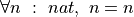 , can be used as a function. It can be applied to a value, n, of type nat, and in this case it promises to returns a proof of the proposition, n = n, for whatever particular value of n it was applied to.
Moreover, to construct a proof of a proposition, we have to show that if we are given an arbitrary value of the quantified type, which is to say an argument, that we can then construct and return a value of the promised return type: a proof of the proposition that comes after the comma. Remember, propositions are types and proofs are values. So we have to show that given any value of the argument type, we can construct and return a value of the resulting logical type, a proof.
We do this by, in effect, constructing a lambda abstraction. That we usually a proof script, rather than ordinary code, is secondary. Here, for example, another way to provide a proof of , 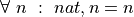 , as a lambda abstraction term.
example : ∀ n : ℕ, n = n :=
    λ k, eq.refl k
As should now be increasingly clear, the connection between proofs of universal generalizations, on one hand, and functions, on the other, is to close that they are … wait for it … the same thing. Indeed, the Lean function type,  is really a shorthand for
  ! A proof, or equivalently, a value, of this type is a function. To prove such a proposition, one must produce a function. To use such a proof, one applies it to a value to obtain a specialized proof for that specific value.
The following example in Lean further confirms what we have just said. If we assume that S and T are arbitrary types, and that pf_all is a proof of , and if we then check the type of this proof, Lean reports it to be . The proof of , and if we then check the type of this proof, Lean reports it to be is a function! If we then assume that x is some value of type, S, and if we apply pf_all to x, Lean tells us that, as predicted, we get a value of type T.
axioms (S T : Type)
axiom pf_all : ∀ (s : S), T
#check pf_all
axiom x : S
#check pf_all x
One sees here, perhaps for the first time in this course, an incredibly close connection between logic and computations. In constructive logic, we have two basic mantras. First, propositions are types. Second, proofs are programs! Moreover, the type checker ensures that all such programs are of the right type: that proofs that are accepted are always valid proofs.
As we’ll see we need to be a bit inclusive when we say that proofs are programs. Some proofs are just data objects. Not every proof is a function. Proofs of “forall” propositions are functions, as are proofs of implications, as suggested strongly by the notation,  .
.
In any case, proofs in constructive logic are terms (values) that we can compute with. This fact is what makes it possible to automate logical reasoning in system such as our Lean proof assistant, in Coq, in Agda, and in other constructive logic proof assistants. We write code that can deal with propositions, predicates, proofs, just as easily as, and indeed mixed in with,code that deals with computational values of types such as bool, string, nat,  , and so forth.
3.3.4. Natural Language
If you were given the task of proving a proposition of the form,  , in another class, you would probably not produce a formal proof in Lean. Instead, you would write an informal proof in mathematical English. You might write something like this. “To prove , we start by assuming that t is some specific but otherwise unspecified value of type T. We will show that P is true for this value. That will effectively prove that P is true for any possible value of t.”
On the other hand, if already has a proof of 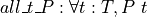 , and if one has a particular value, s, of type T, then it might be useful to derive a proof of
  . One might write, “We know that is true in general so it must be that case that it is true in the specific case where the value of t is s. Thus, from our proof of , we deduce a proof of
  , in particular.
3.4. False
The simplest of all propositions is  . It is even simpler than true, because whereas
  has one constant proof term, true.intro, making it unconditionally true, has no proofs at all, making it unconditionally false.
3.4.1. Formula
In some writing, false is denoted as  , pronounced bottom. In Lean it is just written as false. Check it in Lean using the #check command. False is a proposition. Propositions are types. So false is also a type. And as a type, it has no values. There are no proofs of false. It is an uninhabited type.
#check false
3.4.2. Interpretation
We interpret , as a proposition that can never be proved true. In the constructive logic of Lean, that means that there must be no proofs of it whatsoever.
3.4.3. Introduction Rule
To enforce this interpretation, the type, has no introduction rule. Without an introduction rule, no proof can be constructed. That is what makes false.
3.4.4. Elimination Rule
On the other hand, in a context in which one is assumed to have a proof of , that proof is very handy because from it, a proof of any other proposition whatsoever can be derived. In other words, false being true implies that anything at all is true as well. This idea is formalized in the inference rule called false elimination. Given an assumed proof of and any other proposition, P, one can apply the apply the elimination rule for false to obtain a proof of P. In Lean this rule is called false.elim. Here is the rule in inference rule notation.

You will notice that in writing the inference rule, we enclosed the declaration of the argument, P, in curly braces, rather than in parenthesis. That signals that when we apply this rule in Lean, we will not have to give a value for P explicitly. Rather, the value of P will be inferred from the type of proof to be produced (below the line), which is of course just P.
Here is a short piece of code in Lean showing the application of this rule. Lean supports type inference, and so here, as above, we can surround an argument with curly braces to tell Lean we don’t want to have to specify a value for that argument explicitly, but that Lean should infer the value from context.
1 2 3 4 | def proveAnything ( P: Prop ) (f: false) : P :=
(false.elim f)
axiom bad : false
#check proveAnything (0 = 1) bad
|
What this code shows is that if the proveAnything function were given any proposition, P, along with a proof of false, then it would return a proof of P. Given a proof of false, this function can be used to obtain a proof of any proposition. Lines 1-2 define this function. It takes a proof of , f, and any proposition, P, as arguments, and promises to returns a proof of P, no matter how crazy P might be. Line 3 uses the axiom statement to assume that there is a proof of false, here named, bad. The final line shows that applying the function, proveAnything to this assumed proof of false and to the proposition, (0 = 1), returns proof of (0 = 1). If one has a proof of false, then one can then prove anything at all.
This conclusion, 0 = 1, is absurd, of course. But the assumption that there is a proof of was absurd to begin with. It represents a situation that is impossible. If one finds oneself in such a situation in the course of logical reasoning, then the situation can basically be ignored, as it could not ever actually arise.
Now, you might ask, how can we write a function that takes an argument of a type, false, given that this type has no values? The answer is that such a function definition is fine; it will just never be possible to apply it, as there is no proof of to which it could ever be applied. In writing the body of the function, we can ignore the fact that the function never be applied, and write the code as if arguments of the right types were provided. Within the body of a function, in other words, we assume that arguments of the right types have been given. From now on, think of declarations of the arguments to a function as axioms: facts that can be assumed within the body of the function. This is why we can apply false.elim to an assumed proof of false within the body of our function, even though no such value will ever really exist. Arguments are axioms when it comes to writing function bodies.
You can thus read our function as a piece of logic: if you can provide a proof of false and any proposition, P, this function will give you back a proof of P, no matter what P is. What the existence of this function shows is that  . The function works by applying the false.elim rule. This rule plays a vital role in reasoning about negations: propositions that assert that some state of affairs does not hold.
To conclude, from a proof of false one can derive a proof of anything at all. Logicians have naturally given a latin name to this principle: ex false quodlibet. From false, anything follows. This principle is sometimes also called the principle of explosion. While this inference rule might appear to be of little use since it relies on a proof of , the reader will learn that this is actually a very powerful inference rule that is very useful, for example in proofs by contradiction!
3.4.5. Natural Language
Because there is no proof of , there is no way to give natural language rendition of a proof of the proposition, . If asked to do so, one could simply say, “As there is no proof of false, no proof can be given. The proposition is thus disproved.” On the other hand, if one is in a context in which a proof of false has been derived, and in this context one needs to produce a proof of some proposition, P, one can just say, “from our proof of false, anything follows, so the truth (and a proof) of P, in particular, follows.”
3.5. True
3.5.1. Formula
In predicate and constructive logic, , sometimes written  , and called top, is a proposition. In Lean it is just written as true. Here we use the check command in Lean to confirm that is of type
  . It’s a proposition.
#check true
3.5.2. Interpretation
The intended meaning of this proposition is that it’s unconditionally true. In constructive logic, that means that there must be a proof of true that is always available.
3.5.3. Introduction
To this end, the rules of natural deduction provide one introduction (proof constructing) rule for true. It is called  . It takes no arguments and so imposes no conditions. It can always be used to obtain a proof of .

A function that takes no arguments is a constant. So can be seen as both a function, albeit one taking no arguments, and as a constant. It is a proof of . We confirm this in Lean by checking that the type of true.intro is true. The former is a proof of the latter.
#check true.intro -- true.intro is a proof of true
Here are a few examples using this rule.
lemma t  : true := true.intro     -- explicit type declaration
lemma t'        := true.intro     -- Lean can infer the type
#check t                          -- it's a proof of (type) true
#reduce t                         -- it's true.intro specifically
On the first line we declare the name t to be bound to a value of type, i.e., a proof of, , and we prove that such a binding can be made by providing a proof of to the right of the :=, namely, . The second line shows that we can rely on Lean to infer the type of t, here renamed to t’ to avoid name conflicts. The third line confirms that the type of t is , which is to say that value of t is a proof of this proposition. The final line shows us that the actual proof value is, as expected, .
In the first two lines of the preceding example, we provided the required proofs of by giving a proof value, true.intro, directly in the code. There is another way to provide proofs in Lean, which is often preferable. It’s benefit is that it allows you to construct proof objects incrementally. This technique uses what are called proof scripts to produce proofs. In lieu of an exact proof term, we provide a script enclosed in a begin-end pair. In this case, the script has just one line. It simply offers as an exact proof of true. The name of the tactic in this case is exact. Bring this code up in your browser. Put your cursor on the begin. See how Lean starts by telling you what values you have to work with (none), and what you need of a proof of (true). As you step through the proof script, the obligation to produce such a proof is satisfied.
-- prove lemma by constructing a proof interactively
lemma t'' : true :=
begin
  exact true.intro
end
3.5.4. Elimination
Little of much use can be done with a proof of . There is no elimination rule for true.*
3.5.5. Natural Language
Most working mathematicians and computer scientists still write natural language proofs. To give a (natural language) proof of the proposition, , one could simply say, “The proposition, , is trivially true. QED.” The QED stands for the Latin phrase, quod erat demonstratum, which simply means, “so it is shown.” It’s a traditional way of ending a proof in a way meant to signal that a valid proof is claimed to have been given.
3.5.6. Formalization (Optional)
In constructive logic, propositions are formalized as special types, and proofs of propositions are values of their types. Here is how the proposition, , is defined as a type with one value, that is, one proof, called . We give two definitions, the second of which (with a name change to avoid conflicts)differs only to show that Lean can infer the type of  as
as  . We will prefer to include explicit type declarations in such type definitions.
namespace cs2102

inductive true : Prop
  | intro : true

inductive true' : Prop
  | intro

#check true
#check true.intro

#check true'
#check true'.intro

end cs2102
Consider the first definition, of . The keyword, inductive, introduces a type definition. The name of our type is . It’s type is , which indicates that is a logical type, a proposition, rather than a computational type, such as  or
or  . Following the first line, we define the one constructor for values of this type (for proofs). Each constructor definition for a type is preceded by a vertical bar. The comes the name and type of the constructor. And that is it.
You note that we used the name intro for the constructors in both cases, without any conflicts. That is because each type definition establishes it own namespace, having the same name as the given type. The two intro terms are thus different terms. One is referred to as ; the other, as  . We thus see now exactly where comes from. It is the one and only constructor for values of type , i.e., for proofs of this proposition. Taking no arguments, it is also a constant: the one and only proof of . We will see constructors that take arguments later.
Kevin: see actual Lean libraries to confirm details.
3.6. Conjunction
If P and Q are propositions, then so is . In such a situation, if math:P is true and if is also true, then it must be the case that the proposition, is true and is true, is also true. This intuition is expressed formally in logic using the logical connective,  . It is pronounced and. In Lean, you can create this symbol by typing
 \and followed by a space.
3.6.1. Formula
To formally express the proposition that is true and is true, we write . Such a proposition is called a conjunction. The following code confirms that if we assume that and are propositions, as we do on the first line, then is a proposition. So is and P Q. And these are in fact the same proposition, just written using two different notations.
axioms P Q : Prop
#check (P ∧ Q)
#check (and P Q)
3.6.1.1. Infix, Prefix, and Postfix Notation
The symbol, , appearing between two conjuncts, P and Q, is really just a shorthand notation for the function application term, and P Q. An expression in which an operator (i.e., a function name, such as ) appears between its operands is said to be in infix notation. If the operator in an expression appears before it’s operands, the expression is said to be in prefix notation. Operators can also appear after their operands. Expressions involving the factorial function are generally written in postfix notation. So, for example, the notation, 5!, can be understood as shorthand for the function application term, fac 5. When an operator appears after its operand, the expression is said to be written using postfix notation.
3.6.1.2. Type Constructors
Viewed as a function, and is rather special. It’s a function that takes two propositions, P and Q, which are types, as arguments, and it returns the proposition, the conjunction, and , as a result, which is another type. The operator is another name for this function. We call such a function a type constructor, because it takes types as arguments (remember propositions are types) and returns a type as a result.
As we will see later in more depth, such a type constructor has an associated set of zero or more rules for constructing values of the constructed type. For example, and.intro, is just such a rule. By rule, what we mean is function for constructing values of a type built using a type constructor. We will call such functions value constructors (or, often, just constructors). The and.intro rule is just such a value constructor. It provides a means for constructing proof values for conjunctions (which are propositions and therefore types) that were themselves constructed using the and type constructor.
Be sure you see the essential difference betwen type constructors and value constructors. Here, and, is a type constructor; and.intro is a value, or proof, constructor.
3.6.2. Interpretation
We interpret a conjunction, , as asserting that both and are true. In the logic of Lean, that means there must be a proof of and there must be a proof of . The proof construction rule for conjunctions, i.e., the introduction rule for and, strictly enforces this interpretation.
3.6.3. Introduction
There is one proof construction rule for conjunctions. For arbitrary propositions, and , it constructs a proof of the proposition, . The rules implicitly takes the propositions, and , as arguments, along with a proof,  , of , and a proof,
  , of . It then returns a proof of . Because this is the only value/proof constructor provided with the and type constructor, one simply cannot construct a proof of a conjunction unless one already has proofs of each of the conjuncts. The strict type checking of Lean ensures that this constraint can never be violated. In inference rule notation, here is the and.intro proof construction rule.

Here’s an example in Lean.
axioms P Q R S : Prop
axioms (p : P) (q : Q) (r : R)

lemma pq  : P ∧ Q := and.intro p q

lemma pq' : P ∧ Q :=
begin
  apply and.intro,
  exact p,
  exact q
end

#reduce pq
#reduce pq'
The first three lines assume that P and Q are propositions and that p and q are proofs of P and Q, respectively. Line 5 binds a proof of the proposition, to the identifier, pq. Lines 7-12 do the same thing but with a proof script. The first line in the script indicates that a proof will be constructed by applying the and.intro rule, but no arguments are given. Providing the missing two arguments become sub-goals. One must first provide a proof of P, and exactly p is given. Similarly one must provide a proof of Q, and q is give, completing the proof. The check commands show that the resulting proofs are identical.
EXERCISE: Try to use a proof of  as a proof of . Explain the resulting error message.
EXERCISE: Given the assumptions in this block of code, can you prove  ? Explain why or why not?
3.6.3.1. Pair Notation
You will note that Lean prints out the proof objects for conjunctions using the notation,  . This notation is a Lean shorthand that reflects the fact that the way that we construct a proof of is by providing a pair of proofs, p : P and q : Q. In fact, you can use this shorthand to construct proofs in Lean as the following example shows.
axioms P Q : Prop
axioms (p : P) (q : Q)
lemma pq : P ∧ Q := ⟨ p, q ⟩
EXERCISE: Extend this example to assume that R is also a proposition, and that r is a proof of R. Then use Lean’s shorthand notation for pairs to prove a lemma, that is true.
3.6.3.2. Top-Down, Type-Directed Refinement
In logic as in programming, we can often make a good guess as to what the top-level structure of a proof (or a program) should be, and yet be overwhelmed by the complexity of details needed to finish it off. In such cases, we can employ one of the most important of all software engineering practices: use a top-down, type-directed style of development.
As an example, imagine that we have to prove a conjunction, , and further suppose that proving P is hard and that proving Q is hard. We know that the overall proof term has to be of the form, and.intro _ _, where the first hole is of type P (requiring a proof of P), and the second hole is of type Q. What we can do in such cases is to provide the overall solution but with some remaining holes to be filled in, and then take on the problem of filling each hole as a sub-problem to be tackled separately. This is called top-down development. Every programmer should master this intellectual tool. Moreover, if we’re careful about the types of terms required to fill the holes, and especially if we have a good type checker, which we now do, then we (and the tool) know what form of solution is required in each case. This is what we mean by a type-driven approach to development. Finally, when filling each hole, we then use the same top-down, type-driven approach. At each level, the overall task is thus decomposed into a few smaller tasks, which we can then handle separately in the same manner. In this way, we gain intellectual control over a situation of otherwise overwhelming complexity. The process of filling in details in this manner is known as refinement.
The following example shows how to do it in Lean. We only pretend that proofs of P and Q are hard to obtain in this case. To keep the example simple, we assume them. The example starts by assuming that P and Q are any old propositions. We assume we have proofs of P and Q, but, again, let’s pretend that they’re hard to produce, as in practice they might well be. The first proof (example) in the following logic simply writes out the entire proof term, and.intro p q. But again, if p and q were complex proofs, this term could be long and complex indeed. In the succeeding examples, which we discuss after presenting the logic, we see a fundamental approach to control of complexity in software and proof engineering. We call it top-down, type-directed refinement.
axioms P Q : Prop
axioms (p : P) (q : Q)

example : P ∧ Q :=
    and.intro p q

example : P ∧ Q :=
begin
    apply and.intro _ _,
    exact p,
    exact q,
end

lemma pq : P ∧ Q :=
begin
    apply and.intro,
    exact p,
    exact q
end
EXERCISE: First guess and then confirm what happens if instead of apply and.intro in the third example, we used apply and.intro p. In other words, what happens if we give one of the two required arguments to the and.intro inference rule?
It is important to study these ideas and examples with care, as they illustrates and show the complexity control power provided by a top-down, type-guided, approach to refining complex objects. Asked to produce a proof of a proposition, , where P and Q are themselves complex propositions, we can do it by noting that the proof term that is required has to be of the form and.intro _ _, where the first hole has to be filled with a value of type (a proof of) P, and the second, with a value of type Q. We have thus decomposed the problem of produce a proof of into two simpler problems, though each might itself remain complex,. Once we have recursively produced proofs of these propositions with which to fill the holes, then we will have a complete and working proof that the Lean type checker will accept as a valid term (proof) of the required type (proposition).
In the second proof, we give exactly the same overall proof term–an application of and.intro two two proofs–but now we use holes to delay the refinement of the required arguments, which must be proofs of P and of Q, respectively. Lean now erases the original goal, as it has been satisfied by the overall proof term, contingent on the provision of values of the right types for the two holes. Filling those holes become new sub-goals. One now proceeds recursively to fill the holes. The third example of the same proof below shows that when we use the apply tactic in Lean, we can omit the underscores and Lean will know that we’re simply leaving certain holes unfilled.
We see this principle in action in the proof scripts above. At the start of the script, in a context in which we are assumed to have P and Q as propositions and p and q as proofs, we are to construct a proof of and P Q. To do this, in the first line of the proof script, we use the apply tactic to apply the and.intro proof rule, but, crucially, we omit the two explicit arguments that it requires: a proof of P and a proof of Q. What Lean does at this point is to tentatively accept the proof term, and _ _, with two holes to be filled, as a partially completed proof. Lean then presents the tasks of filling each of the holes, to complete the proof, as two remaining sub-goals. The next line of the script fills the first hole with an exact proof term of the required type, P. The last line fills the remaining hole with a proof of Q. That completes the proof, which Lean accepts as a proof of the original goal.
This approach to developing a complex proof term, a program of sorts, is top-down in the sense that it starts with the kind of proof term needed to prove the overall goal, albeit one with some blanks remaining to be filled in. It is incremental in the sense that one fills in holes one at a time. It is type-guided in the sense that you know precisely what type of term is required for each hole in the partially completed proof term. The idea of top-down, incremental, type-guided development of complex software objects is truly fundamental. A great software developer deeply understands and implicitly practices this approach on a daily and hourly basis.
To be clear, this approach to constructing proofs using top-down, type-guided development in this way can be and should be applied to writing even the most complex of procedures. One starts writing a procedure by writing a top-level program: one that is complete except for the fact that the subroutines that it calls are implemented as stub routines. These are the remaining holes to be filled. When they are filled, then a complete, working program is obtained. Writing code this way, or proofs, allows you to focus on the overall logic of the task to be carried out, while suppressing details that will be elaborated later. One can then reason about whether or not the overall outline is correct without being overwhelmed by the details of the individual sub-goals of filling the remaining holes.
As a simple example, we can develop a function taking two arguments, x and y, of type nat as arguments and returning the sum of their squares. At the top level, the program simply has to compute the sum of two terms. This will be done by applying the nat.add function to two terms. We can ignore the details of these terms in order to establish the overall structure of the program. Then we can fill each of these holes with computations of the squared terms, filling in the initially elided details to complete the task.
Here’s a demonstration of this idea in Lean. First we apply forall introduction, giving names to the two assumed arguments to the program. Then we apply the nat.add (natural number addition function) without specifying its arguments. This leaves us with two remaining holes to fill in; and Lean tells us that they must be filled with terms of type nat. We then recursively develop each of these sub-routines. The first returns the value of x squared. The second returns the value of y squared. Lean confirms that we have constructed a program (a proof of the type “nat to nat to nat”, if you want to think of it that way) by accepting the overall term as having the right type. The #reduce command at the end displays the resulting function as a lambda term, and it’s exactly the function we wanted. This example demonstrates the construction of code in a top-down, type-guided, incremental style of development.
def sumOfSqaures : ℕ → ℕ → ℕ :=
begin
  intros x y,
  apply nat.add,
  exact x*x,
  exact y*y,
end

#reduce sumOfSqaures
EXERCISE: Carry out an implementation of this function in Python or Java or any other industrial programming language. Write a top-level function called sumOfSquares. Have it apply the addition operation to the results of calls to a subroutine called square, that takes a natural number and returns its square. But in the first instance, just have that routine return 0. We call this “stubbing out” a procedure. A stubbed out procedure is a hole in your code. The code must compile and run, though it won’t produce the right answer. You thus have a viable architecture for your program. Now fill in correct implementations of the remaining holes to get to a working system.
The only difference between using a tactic script to develop ordinary functions, on one hand, or proofs, on the other, is the type of term that one is constructing. In our example just prior, we used a tactic script to construct a value of the computational type, nat to nat to nat. Previously, we used a tactic script to develop a value of the logical type, . In each case, we proceded by the method of top-down, structured, incremental, type-guided development.
3.6.4. Elimination
Recall that whereas introduction rules construct proofs, elimination rules give us ways to use proofs to obtain related information. There are two elimination rules for proofs of conjunctions. Given a proof,  , of the proposition , the first rule, called and.elim_left, returns p, the first element of the pair of proofs implicit in a proof of a conjunction. The second inference rule, called and.elim_right returns q, the second element of the pair of proofs.
Here is the first rule. It says that if one is given propositions, P and Q, and a proof of the proposition, , then by applying this inference rule, one can derive a proof of P. The validity of the rule is clear: if we know that both P and Q are true, then it must be the case that P alone is true.

Note that we have used curly braces around the arguments, P and Q. as Lean can infer them from the type of the proof of . When these rules are used in Lean, as you will see just below, the only argument one provides explicitly is the proof of . So, if such a proof is called pq, then an application of this rule will look like  , yielding a proof of P as a result.
Here is the second elimination rule for proofs of conjunctions. It says that under the same conditions, one can also derive a proof of Q.

Here are examples showing the automation of these rules in Lean.
-- let's first build a proof of P ∧ Q
axioms P Q : Prop
axioms (p : P) (q : Q)
lemma pq : P ∧ Q := ⟨ p, q ⟩    -- we have a proof, let's use it

-- now let's use it
lemma p' : P := and.elim_left pq
lemma q' : Q := and.elim_right pq

-- here's one shorthand for and.elim_left and right
lemma p'' : P := pq.left
lemma q'' : Q := pq.right

-- here's an even shorter shorthand
lemma p''' : P := pq.1
lemma q''' : Q := pq.2
EXERCISE: Write a function in Lean that takes two propositions, P and Q, as implicit arguments, along with a proof of , and that returns a proof of  . Once you’ve written this function, apply it to an assumed proof of
  , where S and T are assumed to be arbitrary propositions. What is the type of the result?
3.6.5. Natural Language
If asked to prove a conjunction, a proposition of the form, , where and are smaller propositions, you say something like this: “To prove , we first prove , and then , and with these proofs in hand a proof of will follow.” You can generally assume that most readers know that if you have proofs of both conjuncts, you can produce a proof of the conjunction, so mentioning the inference rule is usually not needed in a natural language proof. Similarly, if one is given a proof of a conjunction as an assumption, one can simple write, “From the truth (or a proof) of the conjunction we can immediately infer the truth (or the existence of a proof) of each of the conjuncts.”
3.7. Implication
In mathematical logic we will often want to state and prove conditional propositions. A conditional proposition, or implication, asserts that if one or more propositions, the premises (or antecedents), are true, then the truth of another proposition, a conclusion (or consequent), is assured.
For example, in everyday language, we might assert that if it’s raining (a premise, a condition), then the streets are wet (a conclusion). In mathematical logic, we might want to formally state and then prove the conditional proposition that if x is even (a premise), and then if y is even (another premise), then  must be is even (the conclusion).
3.7.1. Formula
We state such propositions formally as implications. If P and Q are propositions, we write the conditional proposition, or implication, if P is true then Q is true, using an arrow notation: . We read this proposition as P implies Q, or if P then Q. In Lean you can create the → symbol by typing \to followed by a space. In the following code block we assume that P and Q are propositions, and then we use #check to confirm that is then a proposition as well.
axioms (P Q : Prop)
#check P → Q
3.7.2. Interpretation
When should we judge an implication proposition to be true? The answer to this question is slightly subtle and bears careful explanation.
An implication, , asserts that if P is true then Q must be as well. In other words, it constrains Q to be true if and only if P is true. It imposes no constraint on Q if P is false. The only time that the constraint imposed by an implication is violated is when the premise, P, is true and the conclusion, Q, is false. In this one case, the implication is judged to be false. In all other cases, it is judged to be true in the sense that the constraint it imposes is satisfied.
As an example, the proposition,  is true because the premise is false. From a false premise, anything follows. It doesn’t matter whether the conclusion is true or false. If the premise of an implication is false, then the implication as a whole is always true. On the other hand,
  is false because the premise is true but the conclusion is not.
3.7.3. Introduction
In constructive logic, for a premise of an implication, , to be true means that there is a proof of it. So, what it means for an implication to be true is that if there is a proof of its premise, P, then there must be a way to obtain a proof of its conclusion, Q. Another way to say this is that is true if, whenever one is given a proof of P, or in other words, if one assumes that one has been given a proof of P, which is the case within the body of a function that takes a value of type P as an argument, then it is possible to derive a proof of Q. A way to derive a proof of Q (a value of type Q) from a proof of P (a value of type P) is nothing other than a function, namely one of type .
We thus have our introduction rule for implication. The rule says if we can provide a formula for deriving a proof of Q from any proof of P, then we can conclude, and we have a proof of, the implication . A function that converts proofs of P into proofs of Q is a proof of the implication. A function of type , where P and Q are propositions is a proof of the logical implication, .
In constructive logic, proofs are programs. If P and Q are computational types, such as nat, then the type, , is the type of computational functions from values of type P to values of type Q. If P and Q are propositions, then the function type, , is the type of proofs of the logical implications, . To prove the logical implication, , one must give a value of this type. That value will be a function, from proofs of P (values of type P) to proofs of Q (values of type Q). Propositions are types. Proofs are programs. In the case of implications, proofs are actually functions.
Most of the propositions one needs to prove in practice in mathematics, logic, and computer science will involve implications. The goal is usually to show if certain conditions, formalized as premises, hold, then a certain conclusion must follow. To prove such a proposition, what one generally does is to assume that the premise is true, and to show, in the context of this assumption, that a proof of the conclusion can be derived. Constructing a proof of the conclusion will generally require that one use the assumed the proof of the premise. One thus generally applies elimination rules to the assumed proof of a premise to obtain the elements needed to finally construct a proof of the conclusion. The result is a proof that if there really is a proof of the premise, then a proof of the conclusion can be obtained. If the premise is true, so is the conclusion.
3.7.3.1. Informal Example
Suppose, for example, that we want to prove that if any two natural numbers, n and m are equal to each other, then n + 1 is equal to m + 1. We would formalize this claim with the following proposition:  . This proposition is a universal generalization that asserts that no matter what values n and m have, if n = m then it must be the case that n + 1 = m + 1. It might seem obvious that this is true, but to certify the truth of this proposition, we need a proof. To obtain such a proof we will reason as follows. First, we will assume that n and m are specific but unspecified natural numbers. Second, we will assume that n = m. That means that we assume that we have a proof of n = m. In this context, we must show that n + 1 = m + 1. To do this, we will use our proof of n = m to justify the rewriting of the n to m in the proposition, n + 1 = m + 1. That will yield the proposition m + 1 = m + 1. That in turn is easily proved by appeal to the reflexive property of equality.
3.7.3.2. Formal Proof Construction
lemma incEqual : ∀ n m : ℕ, n = m → n + 1 = m + 1 :=
begin
  intros n m,
  assume neqm,
  rewrite neqm,
end

#check incEqual
#check incEqual 3 3
Here we use a proof script to construct the required proof. In the first step, we use forall introduction. That is, we assume that n and m are specific but unspecified natural numbers. In the second step, we assume that n = m. That is, we assume that the premise of the implication is true, and that we have a proof of it. Be sure to watch how the proof context and goal evolve as you go through the steps of this script.
What now remains to be proved, in the context of the preceding assumptions, is that n + 1 = m + 1. This is proved by using the assumed proof of n = m to rewrite the n in the goal to m. At this point, the rewrite tactic determines that what is left to prove is easily proved by applying the eq.refl rule. It kindly applies it for us automatically to polish off the proof.
The result is that incEqual is now bound to a Lean-checked proof of the proposition: that for any natural numbers, n and m, if n = m then n + 1 = m + 1. The proposition we have proved is not itself an implication, but a universal generalization. This is clear in the report obtained by the first #check command. But recall that a universal generalization is itself a function. If given two values of type nat, n and m, applying the rule for forall elimination, the result is an implication specialized to the specific values that were given. Thus the term (incEqual 3 3) therefore really is an implication, namely that 3 = 3 implies that 3 + 1 = 3 + 1.
Note again that this implication being true does not prove that any two natural numbers, n and m are equal, but only that if they are equal, under an assumption they are equal, then the truth of the conclusion, that n + 1 = m + 1, must follow. For example, if you apply incEqual to the values, 3 and 4, you will get the implication, 3 = 4 implies 3 + 1 = 4 + 1. The implication is true but this is the case because the premise is false, and from an assumed proof of false anything follows.
EXERCISE: Prove that ∀ a b : nat, a = b → b = a.
EXERCISE: Prove that ∀ a b c : nat, a = b → b = c → a = c
That last exercise looks a lot like a proof of transitivity for equality, except one might expect to see it written as  . However, we can prove that for any propositions P, Q, and R, the proposition
  is equivalent to the proposition
  , by showing that each proposition implies the other (a concept we will discuss further in bi-implication):
example: ∀ (P Q R: Prop), (P → Q → R) → (P ∧ Q → R) :=
begin
  assume P Q R,
  assume pfPimpQimpR,
  assume pfPandQ,
  have pfQimpR := pfPimpQimpR pfPandQ.1,
  exact pfQimpR pfPandQ.2,
end

example: ∀ (P Q R: Prop),  (P ∧ Q → R) → (P → Q → R) :=
begin
  assume P Q R,
  assume pfPandQimpR,
  assume pfP,
  assume pfQ,
  have pfPandQ := and.intro pfP pfQ,
  exact pfPandQimpR pfPandQ,
end
3.7.4. Elimination
Given that a proof of an implication is a function, it should now be clear that the way to use a proof of an implication is to apply it to a value of the right kind. Given a proof of , one can apply it to a proof of P to obtain a proof of Q. That is, given a proof, pimpq of , and given a proof of P, p, the application (pimqp p) will compute and return a value of type Q, which is to say, a proof of Q.

There is no named arrow elimination rule provided by the Lean libraries. That said, it would be easy to implement one if desired, as the following code shows.
1 2 3 4 5 6 7 8 9 10 11 12 13 14 15 16 17 18 19 20 21 | def arrow_elim { P Q : Prop } (pimpq: P → Q) (p : P) : Q :=
(pimpq p)
#check arrow_elim
#reduce arrow_elim
def arrow_elim' :
∀ { P Q : Prop },
∀ (pimpq : P → Q),
∀ p : P,
Q :=
λ P Q pimpq p, pimpq p
#check arrow_elim'
#reduce arrow_elim'
axioms S T : Prop
axiom pfImpl : S → T
axiom s : S
#check arrow_elim pfImpl s
#check arrow_elim' pfImpl s
|
We provide two implementations of this rule, one in C style, one in lambda style. Study both carefully. Take note of how we specify that P and Q are to be inferred as implicit arguments. Also, on lines 8 and 12, you will see that we need not write one lambda per argument to a multi-argument function; we can just string together the names of the arguments as a shorthand. Also note that Lean infers the types of all of the arguments from the specified type of the function. At the end of the example, we confirm with #check commands that applying the arrow elimination inference rule (simply a function) works as expected. It is, of course, just a function that takes a function (serving as a proof of an implication) and a value (serving as a proof of its premise) and it applies the function to the value to obtain new value (a proof of the conclusion).
The following example in Lean shows this same concept in action using a proof script. For sake of completeness we start by restating the incEqual lemma from above. This example will require some careful study. Be sure to understand what is the type and the value of each term in this example
lemma incEqual : ∀ n m : ℕ, n = m → n + 1 = m + 1 :=
begin
  intros n m,
  assume neqm,
  rewrite neqm,
end

def use_impl { P Q : Prop } (pq: P → Q) (p: P) : Q :=
    pq p

#check use_impl (incEqual 3 3) (eq.refl 3)
Here we define a function, use_impl, that illustrates the use of a proof of an implication. It does this by assuming that P and Q are arbitrary propositions, by assuming that it is given a proof, pq, of as an argument, and by assuming that it is also given a value, (p : P) as an argument. Within the body of the function, one assumes that this context is established. Given this context, one then obtains a proof of Q simply by applying the proof of to the assumed proof of P. The result is a proof of Q, and that is the type of value that the function promised to return. Lean accepts this function definition as well typed, and so it is confirmed that from proofs of the given premises, and , the desired proof of the conclusion, Q, can always be obtained.
All of this might seem a bit abstract. Consider an example from everyday life. If we accept that if it’s raining then the streets are wet, and if we further accept that it’s raining, then we have no choice but to conclude that the streets are wet. In constructive logic, to accept that if it’s raining then the streets are wet means that one has a proof of this implication. Similarly to accept the proposition that it’s raining means that one has a proof of the premise of the implication, as well. From these two facts, certified by proofs, one can deduce that the streets are wet. From a proof of an implication and a proof of its premise one can always obtain a proof of its conclusion. In constructive logic this is done by applying the proof of the implication, which is a function, to a proof of the premise, which is a value of the type that the function takes as an argument, and what one obtains is a value of the return type, which is to say a proof of the conclusion.
We thus now have an intuitive understanding of the elimination rule for implications. To use a proof of an implication, apply it to a proof of its premise. What you get back is a proof of its conclusion. That’s it!
EXERCISE: Prove that for any propositions, P and Q,  . Hint. You will have to assume that you are given a proof of . You will then have to use this proof to obtain the elements needed to construct a proof of . What rules are available for using a proof of a conjunction?
3.7.5. Assume-Show-From Proofs
Todo
Give better example
Here’s a equivalent tactic script for generating the same proof of 0 ≠ 1.
lemma zneqo'' : ¬ 0 = 1 :=
    begin
        assume h : (0 = 1),
        show false,
        from nat.no_confusion h,
    end
This example introduces what we will call the “assume, show, from” proof pattern. The assume h corresponds to h being an argument of the function we are defining to prove ¬ 0 = 1. The show false states what is to be proved (the “return type”). And the from then provides the function body, the code that actually constructs the proof, using what has been assumed. Be sure to open the Messages View in VSCode, click through the script line by line, and watch how the tactic state changes.
EXERCISE: Determine which of the following propositions can be proved. Express and prove them in Lean.
- true → true
- true → false
- false → true
- false → false
3.7.6. Natural Language
Implications are the most common kind of conjectures (unproven proposition) you will be asked to prove. The reason is that one generally wants to show that if certain conditions hold (if certain premises are true), then certain outcomes are assured (certain conclusions follow).
To write an informal proof of an implication, , one begins with words to this effect: To prove the proposition, we first assume that the premises are true, then in the context of these assumptions, we show that the conclusion must follow.
In some cases, the truth (and in constructive logic, a proof) of an implication will be given as an assumption. For example, you might be asked to prove that, if it’s true that “if it’s raining then the streets are wet”, and if it’s also true that “it’s raining”, then it must be true that “the streets are wet”. The first premise is an implication. To prove the conclusion in this case, one must use the truth of the premise. See the statement of the elimination rule for implications. To use a proof of an implication in an informal proof, you you would say something like this. “We already have proofs that P implies Q and that P is true. So it follows immediately that Q must be true as well.”
As we see here, one need not always quote the inference rule being applied in an informal proof. Educated readers will often see immediately what is going on. If there’s any real possibility of confusion, then one should cite the specific already accepted rule, whether a basic inference rule or an already proven lemma or theorem, that is being used to deduce the truth of a desired conclusion.
3.8. Bi-Implication
If P and Q are propositions, then so is  . We call this form of
proposition a bi-implication or an equivalence or biconditional. Mathematicians tend to pronounce the proposition, , as P if and only if Q. They tend to spell it as P iff Q. That’s not a typo: it’s I F F, and is pronounced as if and only if.
. We call this form of
proposition a bi-implication or an equivalence or biconditional. Mathematicians tend to pronounce the proposition, , as P if and only if Q. They tend to spell it as P iff Q. That’s not a typo: it’s I F F, and is pronounced as if and only if.
3.8.1. Formula
The following code shows how to form a bi-implication. The bi-implication arrow in Lean is obtained by writing \iff followed by a space to trigger the requisite text substitution.
axioms (P Q : Prop)
#check P ↔ Q
3.8.2. Interpretation
An equivalence, or bi-implication, is a proposition. When can we judge such a proposition to be true? It is true precisely when the implication going in each direction is true. In other words, is equivalent to  . In other words,
  .
.
Suppose that is true. What does this mean. We can now figure it out. If is true, then if P is true Q must be, too, and if Q is true, then so must be P. On the other hand, if P is false, then so must be Q, and if Q is false, then so must be P.
Here’s a somewhat silly example: if it has been raining in the desert then the ground in the desert is wet. And if the ground in the desert is wet then (we will assume that) it has been raining in the desert. In this case, we can say that the ground in the desert is wet if and only if (iff) it has been raining in the desert. We do ignore here the real-world possibility of oases!
Compare the following proof that the propositions and are equivalent to the two implication proofs at the end of the Formal Proof Construction subsection in the Implication section:
example: ∀ (P Q R: Prop), (P → Q → R) ↔ (P ∧ Q → R) :=
begin
  assume P Q R,
  apply iff.intro _ _,      -- need proof in each direction
    -- (P → Q → R) → (P ∧ Q → R)
    assume pfPimpQimpR,
    assume pfPandQ,
    have pfQimpR := pfPimpQimpR pfPandQ.1,
    exact pfQimpR pfPandQ.2,
    -- (P ∧ Q → R) → (P → Q → R)
    assume pfPandQimpR,
    assume pfP,
    assume pfQ,
    have pfPandQ := and.intro pfP pfQ,
    exact pfPandQimpR pfPandQ,
end
3.8.3. Introduction
To prove a proposition of the form, , one must prove the implication in each direction. More formally, what one is doing in this case is applying the introduction rule for iff to two proofs: one of and one of  to construct a proof of .
Here’s an example illustrating the use of bi-implication introduction. We assume that if it’s raining then the ground is wet, and if the ground is wet then its raining, then from proofs of these two implications we derive a proof of the bi-implication.
axioms (RainingInDesert GroundWet : Prop)
axiom rw : RainingInDesert → GroundWet
axiom wr : GroundWet → RainingInDesert
example : RainingInDesert ↔ GroundWet :=
    iff.intro rw wr
Here’s the same example a little bit more abstractly.
axioms P Q : Prop
axioms (pq : P → Q) (qp : Q → P)
#check iff.intro pq qp
EXERCISE: Write this rule out in inference rule notation. Include curly braces to show which arguments to the rule can, and arguably should, be made implicit.
EXERCISE: Define a function, iffIntro, in Lean that takes two propositions and proofs of implications between them in each direction, that returns a proof of a bi-implication between them. Write the code in C style. Then show that it works by assuming some propositions and proofs of implications, and show that applying your function to these values yields a proof of the expected bi-implication.
3.8.4. Elimination
A proof of a bi-implication is very much like a special case of a proof of a conjunction. In Lean there are separate inference rules for bi-implications, but they are essentially the same as the rules for and introduction and elimination. We just saw that iff introduction takes two proofs as arguments and, in effect, constructs a proof of the conjunction of the propositions they prove. And as one might now guess, there are two elimination rules for iff. They are called iff.elim_left and iff.elim_right. Each takes (implicitly) two propositions, P and Q, and (explicitly) a proof of . The iff.elim_left rule returns a proof of . The and.elim_right rule returns a proof of .
axioms P Q : Prop
axiom p_iff_q : P ↔ Q
#check iff.elim_left p_iff_q
#check iff.elim_right p_iff_q
EXERCISE: Assume that P and Q are arbitrary propositions. Prove formally that  .
.
EXERCISE Assume that P and Q are propositions. Prove that  . Call your lemma and_commutes. You will have proved that conjunction is commutative: that for any two propositions, P and Q, if is true then so is .
EXERCISE: Extend your work from the previous exercise by assuming that S and T are propositions and that you also have a proof of . Use #check applied to an expression that derives a proof of  from the proof of . Use the lemma you just proved (it’s a function!) Don’t use either
 and.intro or and.elim in your new expression. Lemmas (or theorems), once proved, become new super-inference rules. You can then apply them, just as you’d call a function to carry out a complex task, rather than writing it entirely from scratch each time you need it.
3.8.5. Natural Language
In mathematics, computer science, and logic, one will not infrequently want to prove that two propositions imply each other: that given propositions, P and Q, are equivalent. A natural language proof would start like this: “We are to prove P iff Q. To do so, we first need to prove P implies Q. Then we need to prove Q implies P. We first prove the former. (Then come details of the proof “in the forward direction”.) Now we prove the latter. (Now come the details of the proof in the reverse direction.) Having proved the implication in each direction we conclude that the bi-implication holds. Educated readers will understand why the conclusion follows, but if one wants to be absolutely certain, one could say “by the application of the natural deduction rule of bi-implication introduction.”
EXERCISE: Applying iff.intro in a tactic script without any arguments proposes a proof of a bi-implication with two remaining holes as a proof of the current goal. The two holes are then represented as sub-goals. The sub-goals are naturally the goals of proving the implications in each direction. Prove that zero equals zero if and only if one equals one using a tactic script. Apply iff.intro as the first step. Then complete the proof by proving the implication in each direction. (Hint: To do this, use the strategy for proving implications.)
EXERCISE Prove that  . Be sure you understand where the implied parentheses are in this proposition. You can put them in and use
 #check to see if Lean prints the result as you expect.
EXERCISE: Prove that  .
.
EXERCISE: Can you prove that  ? Why or why not?
3.9. Disjunction
If P and Q are propositions, then  is also a proposition, and is read as P or Q. A proposition of this form is called a disjunction. P and Q are called its disjuncts. Such a proposition is understood as asserting that at least one of the disjuncts, P or Q, is true. In constructive logic, this means that a proof can be given for at least one of them.
3.9.1. Formula
In the constructive logic of Lean, the  operator is an infix notation for the type constructor (and specifically the proposition constructor), called or. It takes two propositions as its arguments and returns the proposition that is their disjunction as a result. The following bit of Lean logic illustrates the formation of disjunctions using both the infix operator and the equivalent function symbol, or. The last line asserts and proves that the two resulting propositions are the same.
axioms (P Q : Prop)
#check P ∨ Q
#check or P Q
example : (or P Q) = (P ∨ Q) := rfl
3.9.2. Interpretation
What we mean to assert with a disjunction, , is that at least one of the disjuncts is true. What the truth of a disjunction, , does not, by itself, tell us is which one is true. From the truth of alone, we thus cannot infer that either of the disjuncts is true. We only know that at least one of them is true.
3.9.3. Introduction
The introduction and elimination rules for disjunction enforce its intended meaning in constructive logic. To construct a proof of a disjunction, , one needs to know that at least one disjunct is true. In constructive logic, that means that one has to provide a proof of at least one of the disjuncts as an argument.
There are thus two introduction rules for disjunctions, one for each of the two possible cases. In the first case, a proof of is constructed from a proof of P. In the second case, a proof of is constructed from a proof of Q. There are no other ways to construct proofs of disjunctions in constructive logic (except by using other functions that ultimately invoke one of these two rules).
The two introduction rules for disjunctions in constructive logic are called intro_left and intro_right. They are defined in the namespace of the or type constructor (about which we’ll learn more later), and so are generally referred to as or.intro_left and or.intro_right.
The rules operate as one would expect. The first constructs a proof of a disjunction from a proof of the left disjunct. The second constructs a proof of a disjunction from the a proof of the second disjunct. There is one subtlety. It concerns implicit arguments.
Here’s the issue. The rule that constructs a proof of from a proof of P, let’s call it p, infers the proposition P from p. However, one does not give a proof, q, of Q as an argument, so the rule has no argument value from which to infer Q. As a consequence, it can’t infer the type of disjunction that is to be proved; it only knows that it’s P or <something>.
Therefore, when you apply or.intro_left you must give it not only a proof of P but also the proposition, Q, as arguments. Similarly, the introduction rule that constructs a proof of from a proof of Q also takes the proposition, P as an first argument. In both cases, the first argument is the proposition for which a proof will not be given. The second argument is a proof of the disjunct for which a proof will be given.
Here is the or.intro_left inference rule followed by an example of its use in Lean.

axioms (P Q : Prop) (p : P) (q : Q)
#check (or.intro_left Q p)
Here is the or.intro_right inference rule with a corresponding example.

axioms (P Q : Prop) (p : P) (q : Q)
#check (or.intro_right P q)
When faced with the task of proving a disjunction, the key move is to select a disjunct for which a proof can to be given. For example, if the disjunction to be proved is  , it will clearly be preferable to pick the left disjunct, as the right disjunct is false and has no proof. Here is a simple example in Lean.
example : 0 = 0 ∨ 0 = 1 :=
  or.intro_left (0 = 1) rfl
In a tactic-based proof construction, the typical pattern is to apply an or introduction rule giving only its first argument, the conjunct that is not to be proven, leaving the construction of the second argument, the proof of the selected disjunct, as a subgoal. What it looks like when such a rule is applied in a tactic script is that the part of the disjunction that is not to be proved is discarded, leaving the disjunct that is to be proven as a remaining goal.
example : 0 = 0 ∨ 0 = 1 :=
begin
    apply or.intro_left (0 = 1),
    exact rfl,
end
Having to give two arguments of different types to these inference rules is a bit tedious and can be confusing. The good news is that Lean can often infer the first argument from the goal to be proved. In such cases, one can use the or.inl and or.inr variants of or.intro_left and or.intro_right giving only the proof of the disjunct to be proved as an argument. As before, in a tactic script, one often omits even this one argument, leaving it as a subgoal to be constructed.
example : 0 = 0 ∨ 0 = 1 :=
  or.inl rfl

example : 0 = 0 ∨ 0 = 1 :=
begin
  apply or.inl,
  exact rfl
end
One is often asked to prove that compound propositions formed using more than one disjuction operation are true. In such cases it’s important to understand that any such proposition is still formed by applying the or operation to two smaller propositions. So the approach is the same: pick the disjunct that is to be proved, left or right, which can now itself be a smaller disjunction. Then repeat the process for the remaining disjunction to be proved until you have isolated the disjunct for which a proof can be constructed.
axioms X Y Z W : Prop
axiom x : X
axiom z : Z

example : (X ∨ Y) ∨ (W ∨ Y) ∨ Z ∨ X :=
begin
apply or.inr,
apply or.inr,
apply  or.inl z,
end
3.9.3.1. EXERCISES
EXERCISE: State and prove the proposition, 0 = 0 or 0 = 1.
EXERCISE: State and prove the proposition, 0 = 1 or 0 = 0.
EXERCISE: State and prove the proposition, 0 = 0 or 1 = 1.
EXERCISE: Try to prove 0 = 1 or 1 = 0 then explain exactly where you get blocked.
EXERCISE: Replace the or.inl in the lemma below with or.intro_left and supply the missing argument:
axioms (P Q: Prop)
lemma pfPorQ: P → P ∨ Q :=
begin
  assume p,
  exact or.inl p,
end
3.9.4. Elimination
Knowing that a disjunction is true tells you that at least one of its disjuncts is true. If all you know is that it’s true, then you know nothing about which disjunct made it true. Suppose that P and Q are propositions and that porq is (or has been assumed to be) a proof of . How can you use this information? This question brings us to the elimination rule for disjunctions.
The elimination rule involves not only a proof of , but two other pieces of information, namely proofs that, no matter which disjunct made true, the truth of some other proposition, R, follows. The elimination rules thus involves not only a proof of but also proofs of  and
and  . If one has all three proofs in hand, then one can deduce that R must be true. One knows that is true, and that R follows in either case (whether P is true or Q is true), so R must be true.
One thus reasons about disjunctions by what we call case analysis. One considers each case in turn. In the first case, one assumes that there is a proof of P that makes true. In the context of this assumption, if one also has a proof of , then one can apply arrow elimination to obtain a proof of R. Then one must consider the other case, that there is a proof of Q that makes the disjunction true. If in this context one can also show that R follows, then one has shown that it follows in either case. Since at least one of the cases must hold (for that is what the proof of a disjunction means), then the conclusion, R, must follow.
The elimination rule formalizes and enforces our informal explanation. To construct a proof of R from a proof of requires two additional arguments: a proof of and a proof of . The first argument shows that at least one of the cases holds. The second and third arguments show that in either case the conclusion, R, follows. The rule then derives a proof of R.
In inference rule notation, the rule is written as follows. Note that the arguments, P, Q, and R are to be given implicitly. When one applies the rule, one does not give them explicitly.

The following code shows formally how or.elim works in principle. On the first line, we assume that P, Q, and R are arbitrary propositions. On the second, we assume we have a proof, porq, of . On the third line, we assume we have proofs of and . These are the ingredients that are needed to be able to apply the or.elim inference rule. On line 4, we confirm that the result of applying or.elim to these three proofs derives a proof of R.
1 2 3 4 | axioms P Q R : Prop
axiom porq : P ∨ Q
axioms (pr : P → R) (qr : Q → R)
#check (or.elim porq pr qr)
|
3.9.4.1. Top-Down Proof Construction
In practice, we will often start with a proof of a disjunction, but we will lack, and will have to develop, proofs of the two required implications. In such a case, we can apply or.elim to just one argument, the proof of the disjunction, leaving holes for proofs of the two implementation. We will then prove these propositions as sub-goals, in a top-down, type-driven manner, to complete the overall proof. The following logic illustrates this idea using a tactic-style proof.
1 2 3 4 5 6 7 8 9 10 11 12 13 14 15 16 17 | axioms P Q R : Prop
axiom porq : P ∨ Q
axioms (pr : P → R) (qr : Q → R)
-- tactic style proof leaving two arguments as subgoals
example : R :=
begin
apply or.elim porq, -- leave remaining two arguments as subgoals
-- Prove P → R
exact pr,
-- Prove Q → R
exact qr
end
-- term-style proof
example : R :=
or.elim porq pr qr
|
In the preceding example, we start with the same basic assumptions as in the last example. Line 5 then asserts that, in the given context, we can produce a proof of R. The rest of the example constructs a proof of R by top-down, type-driven, development. We start by specifying that an or.elim term will serve as as proof of R. Line 7 does this by applying or.elim to the proof of , leaving proofs of and as holes: as remaining arguments to be provided. Lean accepts the proof conditional on the achievement of two new sub-goals. Each requires a proof of one of the implications. The remaining two tactics provide exact proof terms for these proofs. In a real development, completing each of these sub-goals could be quite complex. At the end of this example we present a term-style proof that makes clear what proof term the tactic script constructed. There’s nothing magical about tactic scripts; they just use convenient programs to construct proof terms that, in principle at least, could be given directly as proof terms.
3.9.4.2. Proof by Explicit Case Analysis
Consider the preceding example but suppose one didn’t already have proofs of the two implications given as assumptions. One would have to construct each of the proofs. To do so for the first case, where one needs a proof of , one would assume P and then show that a proof of R could be constructed. For the second case, one would assume a proof of Q, and in this context show that a proof of R could be constructed.
Lean’s cases tactic further automates this case analysis style of reasoning. It is important to understand that it does nothing other than to automate some aspects of the application of the elimination rule.
axioms P Q R : Prop
axiom porq : P ∨ Q
axioms (pr : P → R) (qr : Q → R)
example : R :=
begin
  cases porq with p q,
    -- Case when P is true
    exact (pr p),   -- shows that a proof of R can be constructed in first case
    -- Case when Q is true
    exact (qr q),   -- shows that a proof of R can be constructed in second case
end
In Lean, one reasons from a disjunction by case analysis. A convenient way to this this is by applying the cases tactic to a proof of a disjunction, leaving proofs of the required implications to be constructed interactivey. Lean then sets up the two cases as subgoals. In the first case, the goal is to show R given an assumed proof of P. In the second case, the goal is to prove R given an assumed proof of Q in the context.
The cases tactic is applied to a proof of a disjunction with an optional with <p> <q> clause, giving the names that should be used for the assumed proofs of P and Q in the two cases. You can use any names you want here as long as they are not already in use. We recommend that when you need to use a proof of a disjunction, you do so using the cases tactic.
EXERCISE: Redo the prior proof, but change the names used after the with in the cases tactic from p and q to proof_of_P and proof_of_Q, respectively, and make any necessary follow-on changes as required to complete the proof.
EXERCISE: Prove the following proposition by case analysis using Lean’s cases tactic.
example: ∀(x : nat), (x = 3 ∨ false) → x + 1 = 4 := _
EXERCISE: Prove by case analysis that (P or false) implies P, again using Lean’s cases tactic.
example: ∀(P : Prop), P ∨ false → P := _
3.9.5. Examples
Here are examples illustrating the preceding ideas.
3.9.5.1. Homing In On the Disjuct to be Proved
Here are a few examples applying or introduction rules to home in on the disjunct to be proved, in cases where this disjunt to be proved is one of several in play.
example : Y ∨ (Z ∨ X) :=
begin
apply or.inr,
apply or.inl z,
end
example : (X ∨ Y) ∨ (W ∨ Y) ∨ Z ∨ X :=
begin
apply or.intro_right (X ∨ Y),
apply or.inr,
apply  or.inl z,
end
example : (X ∨ Y) ∨ (W ∨ Y) ∨ Z ∨ X :=
begin
apply or.inr,
apply or.inr,
apply  or.inl z,
end
3.9.5.2. Different Styles of Proof Using Or Elimination
To apply or elimination, you need to have three elements: a proof of a disjunction, a proof that its first disjunct implies that some other propositions is true, and a proof that its second disjunct also implies that proposition. With these three elements in hand, one can apply or.elim to construct a proof of that other proposition.
axioms ItsRaining SprinklerOn GrassWet : Prop
axiom rs : ItsRaining ∨ SprinklerOn
axiom rw : ItsRaining → GrassWet
axiom sw : SprinklerOn → GrassWet
example : GrassWet := or.elim rw rw sw
In the context of the three given assumptions, it should be clear that the it’s valid to deduce that the grass is wet.
It is important to understand how to use the or.elim rule, both explicitly, as in the preceding example, and implicitly, by using the cases tactic.
The first example below illustates the explicit use of or.elim. The second example recapitulates the first, but now using the “cases” tactic instead of explicit application of or.elim.
You should study the relationships between these two examples carefully and undersatnd exactly what the cases tactic is doing, and how it’s a somewhat easier way to use or.elim followed by assumption of the premises of two implications.
axioms ItsRaining SprinklerOn GrassWet : Prop
axiom rs : ItsRaining ∨ SprinklerOn
axiom rw : ItsRaining → GrassWet
axiom sw : SprinklerOn → GrassWet

example : GrassWet :=
begin
apply or.elim rs,
assume h,
exact (rw h),
assume h,
exact (sw h),
end

example : GrassWet :=
begin
cases rs,
exact (rw h),
exact (sw h),
end
3.9.5.3. Disjunction is Commutative
Now that you understand these rules, you can use them to prove that disjunction is commutative and associative. Here’s a hint: use elimination rules before trying to use introduction rules. If you apply introduction rules too early, you might get stuck.
example : ∀ P Q : Prop, P ∨ Q ↔ Q ∨ P :=
begin
intros P Q,
split,
assume porq,
cases porq with p q,
exact or.inr p,
exact or.inl q,
-- the rest of this proof is left as an exercise for the reader
_
end
3.9.6. Natural Language
Disjunctions are a natural way to think about a world where you know one thing or the other must be true: my keys are in my pocket or they are on the key rack. They are also useful when talking about conditions required for something else to happen: if my keys are in my pocket or if they are on the key rack, then I can find them quickly.
In computer science, it is common to see an if clause similar to: if (A or B) then <do something>. If we are writing safety-critical code we may wish to prove that <do something> only happens if a pre-condition C is true. In this case we would want to prove that  . I.e., we need to prove that the disjunction of A or B implies that C will be true.
3.9.7. Exercises
- Finish the following two proofs.
example : ∀ P : Prop, P ∨ true :=
  _

example : ∀ P : Prop, true ∨ P :=
  _

example : ∀ P : Prop, false ∨ P ↔ P :=
  _

example : ∀ P : Prop, P ∨ false ↔ P :=
  _
- Formalize the following logic in Lean. Let Raining stand for the proposition that it is raining outside. Let Sprinkling stand for the proposition that the sprinkler is running. Let Wet stand for the proposition that the grass is wet. (Assume that they are propositions.) Suppose that if it is raining, the grass is wet. Further suppose that if the sprinkler is sprinkling, the grass is wet. Finally, assume that it is either raining or the grass is wet (but you don’t know which one). In the context of these assumptions, prove that the grass is wet.
-- your code here
3.10. Negation
3.10.1. Formula
In propositional, predicate, and constructive logic, if P is a proposition, then so is  . This proposition is pronounced, not P, and is said to be in the form of a negation. For example, if JoeIsFromCharlottesville is a proposition, then so is
  What the latter is intended to assert is that Joe is not from Charlottesville.
3.10.2. Interpretation
The intended meaning of is the proposition, P is not true, or equivalently that P is false. What it means for a proposition, P, to be false in constructive logic is that there is no proof of P; for if there were a proof of P, then P would be true. In constructive logic, then, it is the proven non-existence of a proof of P that proves that is true.
The question, then, is how to prove that there can be no proof of a proposition, P. The key idea is that if is true, then an assumption that there is a proof of P * would give rise to a contradiction,  , and, as we will see shortly, from a contradiction, a proof of false can be derived. As there is no proof of false, the assumption that there is a proof of P must be wrong, so there must be no proof of P, and
  , must be true. In other words, if
  is true, then there must be no proof of P, and so must be true as well. Indeed, in constructive logic, is defined to be the proposition, .
axiom P : Prop
#print not
#reduce ¬P
It is important at this point to stop and think hard about why this makes sense. What does it mean for to be true? A proof of an implication is a function that assumes a proof of the premise and shows that, in the context of that assumption, a proof of the conclusion can be constructed. How exactly does the truth of this proposition guarantee the non-existences of a proof of P?
3.10.3. Introduction
To show that is true, one shows that an assumption that there is a proof of P enables one to construct a proof of false. In other words, one proves the implication, .
A proof of an implication takes the form of a function: a function that, if applied a proof of P as an argument, returns a proof of false. Having such a function proves that there can be no proof of P, because otherwise it would be possible to construct a proof of false. Again, it is the existence of a function of type that proves the non-existence of a proof of P.
-- Let P be any proposition
axiom P : Prop

-- Now assume that you have a proof of ¬ P
axiom np : P → false

/-
In this context, we can show that if we
further assume that we are given a proof
of P, then we can construct of a proof of
false. We give two versions of the logic.
-/
def noContra (p : P) : false := (np p)

theorem noContra' : ¬ P → P → false :=
    λ np p, (np p)
The idea that a proof of is a function from P to false should be clear in the preceding example. On the first line, we assume that P is any proposition. On the second, we assume that we have a proof of . In this context, we show that assuming that one is given a proof of P, here as an argument to a function, enables one to construct and return a proof of false.
Within the body of the function, we have a contradiction: the assumption made on line 1 that not P is true, and the assumption, made by the declaration of the argument, that we also have a proof of P, enables us to derive a contradition. The function application term (np p) applies a proof-of-not-P function to a proof of P, yielding a proof of false.
From a proof of false, anything at all follows by the application of the principle of false elimination. So in fact, in a context of inconsistent (contraditory) assumptions, one can prove anything at all. First, derive a proof of false, then apply the principle of false elimination. Here we show that if is true, then further assuming that P is true allows one to construct a proof of anything at all. In the following example, from an inconsistent context we prove 0 = 1.
axiom P : Prop
axiom np : P → false
def ifPThenChaos (p : P) : 0 = 1 :=
    false.elim (np p)
3.10.3.1. Proof by Negation
We can now see that we have a general strategy for proving propositions of the form, : We call it proof by negation. To prove not P in a given context, we first assume that we P is true and we show this leads to a contradiction (and thus to a proof of false). We then conclude that P is cannot be true, so not P is true, and P is said to be false.
A classic example of a proof by negation is a proof that the square root of two is irrational. You have to analyze the English a little. This is really the negation of the proposition that square root of two is rational. To prove it by negation, we assume that the square root of two is rational. From that assumption we show that it is possible to derive a contradiction. From that, we then conclude that the square root of two is not rational. And now you have proved it is irrational.
EXERCISE: Prove by negation that the square root of two is irrational (don’t try this in Lean). Start by assuming that it is rational. Hint: if the square root of two is rational, then it can always be written as a ratio of two integers, a / b in reduced form. By reduced form, we mean that a and b are relatively prime: they have no common factors. Common factors in a numerator and denominator can always be cancelled out, leaving a ratio in reduced form. Show that the assumption that you can write the square root of two as a ratio of integers in reduced form leads to a contradiction.
3.10.3.2. Principle of Non-Contradiction
In logic, the principal of non-contradiction states that it isn’t possible to deduce from consistent assumptions that a proposition, , and its negation, , are both true. A context in which both are judged to be true is said to be inconsistent. The false elimination rule enables one to dismiss such situations without further effort.
We can formulate and prove the validity of a universal generalization that expresses this principle of non-contradiction. It states that from a logical inconsistency, a proof of false can be derived, which is enough to show that unless inconsistent assumptions have been made, contradictions cannot occur.
theorem non_contradiction : ∀(P: Prop), (P ∧ ¬P) → false :=
begin
  intro P,
  assume h,
  have p, from h.left,
  have np, from h.right,
  show false, from (np p)
end
EXERCISE: While show false, from (np p) makes it clear that one is deriving a proof of false from contradictory hypotheses, there is an easier way to type it in Lean. Replace that last line with the single tactic, contradiction. This tactic looks for a pair of contradictory hypotheses in the context, and if it finds one it does automatically what you would otherwise type by hand, to derive a proof of false and apply false.elim.
It is important to be able to work with proofs of false. They can’t exist outside of context in which contradictory assumptions have been made, but within such a context, such proofs can be derived, and, moreover, deriving them, followed by the use of false elimination, is exactly the way that one in effect dismisses such a context as not requiring further consideration. In proofs of complex conjectures by case analysis, it often happens that some cases can be dismissed precisely because they contain such contradictions.
3.10.3.3. Axioms and Inconsistency
One the most consequential cases of an inconsistency in the axioms of a logic occurred in 1902 when the British Philosopher, Bertrand Russell, found a contradiction in the logic that the logician, Gottleb Frege, had relied upon in his attempt to define logical foundations for all of mathematics. Frege’s great work was at the publisher when Russell wrote to him with bad news, presenting him with what is now known as Russell’s Paradox.
Russell’s Paradox flowed from the under-constrained way in which Frege’s logic allowed sets to be specified. The result was that in his logic it was possible to define the set of all sets that don’t contain themselves. What Russell (along with several others) asked was whether the set of all sets that don’t contain themselves contains itself. The problem is that if it does, then it doesn’t, and if it doesn’t then it does (think about it!). That’s a contradiction.
This incident convinced logicians that great care would have to be taken to assure the consistency of the axioms of a given logic, in this case the axioms of set theory on which they sought to establish foundations for all the rest of mathematics.
Here’s a single line of logic that shows how easy it is to make inconsistent assumptions. In one line we see the contradiction. In a few hundred pages of logic, or in a set of axioms with complex and subtle interactions, it might not be so obvious that an assumption without proof might cause a contradiction somewhere else in the logic.
axioms (P : Prop) (p : P) (np : not P)
One must be careful when adding axiomatic assumptions to a logic. Whether or not adding an axiom to a logic causes an inconsistency or not turns out to be an important question in mathematics, logic, and computer science. As we’ve already said, the difference between constructive and classical logic is that the latter includes the law of the excluded middle as an axiom, while the former does not. It is known that this axiom is independent of the rest of the constructive logic, and so can be added, or not, without causing inconsistencies.
3.10.3.4. Constructive vs. Classical Mathematics
As an example, a major divide in mathematics is between constructive and classical mathematics, reflecting varying levels of willingness to accept proofs that certain mathematical objects exist. In constructive mathematics, to show that an object that satisfies a certain predicate exists, one must actually show such an object along with a proof that it has the specified property. In classical mathematics, proofs that certain things exist can be accepted even if one cannot actually put one’s hands on (i.e., show a specific example of) such a thing.
Whether one is a classicist or a constructivist, then, is reflected in part by one’s acceptance or not of the so-called axiom of choice. Informally speaking, this axiom allows one to assume that a set can be formed by choosing one element from each of an infinite collection of other sets. This axiom is independent of the other axioms of Zermelo Frankel set theory and so can either be accepted or rejected, yielding two different logics.
Accepting it, which is what most mathematicians do, enables important theorems to be proven. On the other hand, some of the theorems that can then be proven are bizarre. The so-called Banach-Tarski Paradox is a theorem of everyday mathematics that shows that a 3-dimension ball can be broken up into parts that can then be reassembled into two balls just like the first one!
From this example, one can perhaps see why a constructivist school of mathematics arose. The constructive logic of this course evolved from work that eas meant to establish logical foundations for constructive mathematics. You can escape from the constraints of constructivity in Lean simply by adding axioms to the logic.
We will soon see a clear example in the addition of a single axiom that converts Lean into a classic logic proof assistant. The single new axiom is called the law of the excluded middle, and it allows one always to accept a proposition of the form  to be true even if one doesn’t have a proof of either disjunct.
3.10.3.5. Proofs of Inequalities
An important kind of negation in mathematical logic is an inequality. An inequality is a proposition of the form,  . By this notation, we mean
  . To prove we recall that it means , and that this, in turn, means
  . To prove we thus use proof by negation. We assume the premise,
  , and show it leads to a contradiction.
First, we confirm that , , and all mean the same thing.
example : (0 ≠ 1) = (¬ 0 = 1) := rfl
example : (¬ 0 = 1) = (0 = 1 → false) := rfl
To prove by negation, we thus understand it to mean . To prove this implication, we assume the premise and show that in that context the conclusion is true. We thus assume  and show that this leads to a contradiction. Here’s a simple example. We explain the use of the cases tactic in the paragraphs that follow.
example : ¬0 = 1 :=
begin
  assume h,
  cases h,
end
On the first line, we assert that zero does not equal one. We mentally recognize this as stating an implication with premise 0 = 1. The first line of our proof assumes the premise, leaving the conclusion, false, to be proved. This is done on the second line of the tactic script by applying the cases tactic to the assumed proof, h, of 0 = 1. Without getting into details at this point, we can say that Lean recognizes that there are no constructors that could possibly produce a proof of 0 = 1. There’s no way to obtain such a proof (remember the only way to prove an equality is with eq.refl and it only takes one argument). So from an assumed proof of this impossibility, Lean derives a proof of false by case analysis. That finishes the proof that the assumption that 0 = 1 leads to a contradiction, allowing us, and Lean, to conclude that the assumption was wrong, its negation must be right, and so, indeed, it is true, that .
Here’s a more interesting example, showing that for any natural numbers, a and b, the conjunction, a equal b and a does not equal b is always false. We use the example to introduce a few nice constructs in the Lean tactic scripting library.
example : ∀(a b: ℕ), ¬((a = b) ∧ (a ≠ b)) :=
begin
    intros a b,
    assume pfBoth : ((a = b) ∧ (a ≠ b)),
    have pfEq  : (a = b) := pfBoth.left,   -- short for left elim
    have pfNeq : (a ≠ b) := pfBoth.right,  -- same for right elim
    have f     : false, from (pfNeq pfEq), -- now a proof of false
    assumption                             -- and that proves it
end
The proof proceeds as follows. The proposition is a universal generalization, so we introduce previously unused names for arbitrary values of the specified types. Here we use the same names, a and b, as used in the proposition to be proves. This isn’t necessary, but we find that it makes it easier to understand proofs. As a little exercise, rewrite the proof giving different names on the intros line. Note that the intro tactic gives a name to one quantified value, while intros (plural) me be used if giving names to more than one on the same line.
The remaining goal is an inequality and thus an implication. The second line of the proof script (or tactic script) assumes the premise of the implication. The name pfBoth is given to the assumed proof of the premise. Lean shows that we are now working in a context with three assumptions: a and b are arbitrary but specific natural numbers, and pfBoth is a proof of the conjunction.
On the third and fourth lines, we apply the and elimination rules, using the shorthand forms, .left and .right, applied to pfBoth, to obtain proofs of the individual conjuncts. The have tactics bind names to these smaller proof objects. First, we bind the name, pfEq, to a proof of a = b. Second, we bind the name pfNeq, to our proof that a does not equal b. These definitions are added to our context, giving us new elements to work with as we try to reach our goal.
In the next line, we obtain, and bind the name, f, to a proof of false. It is obtained in turn by applying the proof of a does not equal b (a function) to the proof of (a = b). This is an example of the general strategy we introduced above: from any proposition, P and its negation we can alway immediately derive a proof of false.
We also illustrate another syntactic feature of Lean here: the have x : T, from E syntax. Rather than using := followed by a proof term, we use the word from. This keyword is often used when what follows is an inner begin … end tactic script that constructs a term that might be too complex to type to the right of a “:=”. Note that we now also have f, a proof of false, as an assumption in our context. The final line tells Lean to prove the goal, which is now just false. The assumption tactic searches the context for an assumption that immediately proves the goal. Lean finds f, uses it, and accepts that the overall proof term that we have constructed in an incremental manner with our script is a valid proof of the original proposition.
EXERCISE: Prove that “Hello, Lean!” ≠ “Hello Lean”? Note that when the Lean IDE puts an orange line to the left of certain lines of logic, it means that the Lean prover is working in the background. It might actually take Lean a few seconds to process a proposed proof in this case. Automated checking of large or complex proofs can take quite a bit of time.
EXERCISE: Prove 2 ≠ 1?
EXERCISE: Prove the principle of non-contradiction by formulating and proving the proposition that, for any proposition, P, the proposition, P and not P is false. Do this without looking back at the notes!
EXERCISE: Prove that for any natural numbers, a and b, a equals b and a does not equal b is false.
3.10.3.6. Modus Tollens
We now turn to an ancient and famous inference rule called modus tollens. We start with an example to give a sense for why the rule makes sense.
Assume that if it’s raining, the streets are wet. Now assume in addition that the streets are not wet. What can you deduce about whether it is raining or not? Of course the answer is that it must not be raining, for we have already accepted that if it were raining then the streets would be wet.
There is a general reasoning principle, or inference rule, at play here. It is often called it modus tollens. The principle states that from an assumption, , it is valid to infer that if the conclusion is false, then the premise must be, too:  . The overall rule then says that if the implication, is true, then must be, too. In other words,
  . Another way to parse this proposition is as asserting that if P implies Q and Q is false, then P must be false as well.
In the following example, we first state and prove the principle of modus tollens in general, then we show how we can apply this theorem in a particular setting, where we’re reasoning about rain and streets being wet or not.
-- statement of the theorem in general terms
theorem modus_tollens :
    ∀ { P Q : Prop }, (P → Q) → (¬ Q → ¬ P) :=
begin
  intros P Q,
  intro pq,
  intro nq,
  intro p,
  have q := (pq p),
  contradiction,
end

-- application of the theorem to specific conditions
axioms ItsRaining StreetsWet : Prop
axiom rw: ItsRaining → StreetsWet
example : ¬StreetsWet → ¬ItsRaining :=
begin
    exact (modus_tollens rw),
end
The proof of the modus_tollens theorem in this example is a proof of an implication involving universally quantified variables, P and Q. You can think of (and use) this proof as a function. It accepts arbitrary propositions, P and Q, and a proof of , and gives you back a proof of . A proof of a general theorem thus becomes a highly reusable object! You can apply it anywhere where you have the right arguments.
As an example, assume that one has two propositions, it’s raining and the streets are wet, along with a proof of the proposition that if it’s raining, then the streets are wet:  . In this context, we can apply the modus tollens rule to obtain a proof of the proposition that if the streets are not wet, then it’s not raining;
  . Notice that in the second part of the preceding example, we literally apply the proof of modus_tollens as if it were a function, because it is one! We have a proof of the premise; we need a proof of the conclusion
The following logic first proves that the general principle is valid, giving the resulting proof the name, modus_tollens. We formalize the principle as a universal generalization, quantified over any two propositions, P and Q. The second part of the example illustrates a fundamental point in mathematics that can now be stated explicitly: once we have proved a theorem in a general form, we can apply it to any particular instance we might face, so as not to have to give the entire proof again for that particular instance. What we are doing in such cases is simply applying the rule of universal elimination, to derive a proof of a specific case from a proof of a universal generalization.
EXERCISE: Give a proof of modus_tollens in general form using a lambda-style proof term rather than with a tactic script. Then show that you can apply the result of the weather example.
EXERCISE: Give a proof of modus_tollens as a C-style program rather than using a lambda abstraction directly.
EXERCISE: Is it true that  , or is this a logical fallacy? Try to prove it. Do you get stuck? If you believe the rule is not valid, give a version of our “streets wet” scenario that serves as counterexample to show that the rule, as stated, is not logically valid.
3.10.4. Negation Elimination
What does it mean to say that it’s not not raining? In classical logic, it implies that it’s raining. Double negations cancel. In symbols, we would write  . This is the elimination rule for negation elimination in natural deduction in classical logic. It serves to justify double negation elimination. It might come as a surprise that double negation elimination is not a valid rule of reasoning in constructive logic. If we true to prove it, we get stuck, as we see in the following attempted proof.
3.10.4.1. Negation Elimination is Not Valid in Constructive Logic
example : ∀ (P : Prop), ¬ ¬ P → P :=
begin
intro P,
assume nnp,
-- stuck, no way to make any further progress
sorry
end
To understand what goes wrong here, consider once again what a proof of means in constructive logic. If means that there is no proof of P. so what  means is that there is no proof of :math:`neg P`. But that does not affirmatively tell us anything about whether there is a proof of *P or not, and it certainly doesn’t tell us where to find one!
3.10.4.2. The Middle State in Constructive Logic
This conclusion takes us to one of the most interesting and important aspects of constructive logic: there are not two but three possible states of knowledge about the truth of a given proposition, P. We can have a proof of P, in which case we judge it to be true. We can have a proof of , in which case we can judge not P to be true. Or we can have a proof of neither P nor of . In this middle state, we just don’t know either way.
Such an indeterminate state occurs whenever we have an open (unresolved) problem in mathematics. As an example, consider what is widely seen to be the most important open problem in computer science. It is the conjecture (proposition) written as P = NP. Here P and NP are not propositions. Rather, they are kinds of problems that computers might be used to solve. The proposition is that two classes of problems are actually the same class. To get more to the point, if conjecture is true then there is an efficient algorithm that can solve a certain kind of problem for which we have no efficient algorithm today.
An example of such a currently hard-to-solve problem is that of deciding whether a given graph contains a Hamiltonian cycle. A graph, in this context, is like a map of towns and roads that connect them. A hamiltonian cycle is a path through such a graph (think of a road trip) that visits every town exactly once that that returns to the starting point.
A graph with n towns can have a number of paths that is an exponential function of n. That is, the number of paths can be proportional to  . To decide whether or not there is a path that is a Hamiltonian cycle in a given graph, the best algorithms we have today have to check every possible path in at least some graphs. That means that the time it takes to solve such a problem is also exponential in the size of the problem to be solved (the number of towns), because a computer will have to spend some time computing and checking each path.
An algorithm that takes exponential time is generally considered to be inefficient. A problem for which we have only inefficient algorithms is generally considered to be intractable. A graph with twenty towns won’t be hard to solve. There could be about a million ( ) paths. A fast computer will make quick work of such a problem. On the other hand, a graph with only five times has many nodes (a hundred towns) is a whole different matter. Such a graph could have upwards of
  paths. Thats about 10 followed by 30 zeros, which is an octillion more paths that in the size-20 problem. Exponential functions stay small for a little while and then very big very fast. No real-world computer could even begin to solve such a problem.
The Hamiltonian Cycle problem is one for which it would be tremendous to have an efficient algorithm, especially if one is, say, a delivery company that wants to find delivery routes efficiently. If fact, if we had an efficient algorithm for this problem, we could use it as a subroutine to create algorithms to solve a broad range of important computational problems of great practical value.
So is there a more efficient algorithm? The answer is that today we just don’t know. We don’t have a proof that there is a more efficient algorithm (otherwise we’d probably be using it). Nor do we have a proof that there isn’t one. So we are in this indeterminate middle state, in which we don’t have certain knowledge either way. We don’t have a proof of the proposition,  . Nor do we have a proof of
  . We just don’t know either way.
Consider another example. Most people, sitting in a closed room would agree that it is raining outside or it is not raining outside. If we use X as a shorthand for the proposition, it’s raining, then what we said is that most people would agree with the proposition,  . Applying this idea to the P = NP example, we see that most people would agree with the proposition,
  . Either there is, or there isn’t, an efficient algorithm for solving Hamiltonian Cycle problems.
Now consider what’s needed to construct a proof of in constructive logic. There are two ways to do it. One can apply the left or introduction rule to a proof of X, or one can apply the right or introduction rule to a proof of  . But one has to have a proof of at least one of the disjucts to construct a proof of a disjuction. We don’t have a proof of P = NP today; nor do we have a proof of ; so we have no way to construct a proof of
  .
.
Translating back to the person sitting in the closed room, if she employs constructive reasoning, she could not say that she has a proof that “it is raining or it is not raining”, because she does not have a proof one way or the other. She can’t form a proof of a constructive disjuction. The best she can say is “I don’t have evidence either way.” She is this indeterminate, middle, state of knowledge.
3.10.4.3. Excluding the Indeterminate Middle State
What most people implicitly assume is that a proposition of the form, is true no matter what proposition X stands for. They take for granted the truth of a proposition such as, it is raining or it is not raining outside. Such people use what we call classical logical reasoning. This logic differs from constructive logic by the addition of just a single axiom. It is often called the law of the excluded middle. What is says is that, for any proposition, P, is true. One need not have a proof of either P or of to accept as true. One accepts this fact axiomatically.
In constructive logic, by contrast, to construct a proof of a disjunction requires a a proof of one of the disjuncts, and, in effect, contains a proof of one of the disjuncts. So if we’re given such a proof (other than one accepted axiomatically), we can figure out whether it contains a proof of the left disjunct or of the right one:, and we can even recover and use that proof. Such constructive proofs are thus said to be informative. By contrast, accepting that is classically true tells one nothing at all about which disjunct is true, or why.
3.10.4.4. Classical Reasoning in a Constructive Logic
The question we now ask and answer is whether one can reason classically in a constructive logic, such as the logic of the Lean Prover. The answer is yes. All one needs to do is to assert the law of the excludded middle as an axiom. That is, one asserts that there is a proof ot it. We use the name em (for excluded middle) for this axiomatically accepted proof.
axiom em : ∀ (P : Prop), (P ∨ ¬ P)
This axiom is in the form of a universal generalization, which means that one can apply it to any particular instance of P to get a proof of for that particular instance. We can see this in the following example. We take ItsRaining to be a proposition and apply em to it to instantly obtain a proof of the proposition,  .
.
axiom ItsRaining: Prop
axiom em : ∀ (P : Prop), (P ∨ ¬ P) -- excluded middle
def rornr : ItsRaining ∨ ¬  ItsRaining :=
        em ItsRaining
#check rornr
We call em the laws of the excluded middle because it rules out the indeterminate middle state in which we don’t have a proof either way, by allowing us to assume that either there is a proof of P or a proof of . That is, there are only two remaining cases and at least one of them has to hold.
3.10.4.5. Excluded Middle Enables Negation Elimination
We started this section by asking whether we can assume that the negation of the negation of a proposition P implies P in constructive logic. We found that the answer was no. What we now show is that if we accept the law of the excluded middle, em, then .
example :
  ∀ (P : Prop), P ∨ ¬ P → (¬ ¬ P → P) :=
begin
intro P,
assume pornp,
assume nnp,
cases pornp with p np,
assumption,
contradiction,
end
First, the proposition is an implication. The premise is simply the law of the excluded middle. To prove the implication, we accept it as an assumption. In the context of this assumption, we show that the conclusion follows, and the conclusion simply asserts from the negation of a negation of P we can deduce that P is true. The first line of the proof script uses forall introduction to assume that we have a specific proposition P to work with. The second line assumes that we have a proof, pornp, of the premise. The third line assumes that we have a proof of the premise of the conclusion, i.e., that we have a proof of not not P. In this context, we need a proof of P.
The crucial move here is touse the law of the excluded middle applied to P to obtain (for free) a proof of P or not P. This is a powerful move because it rules out the possibility of a middle, indeterminate state. By giving us a proof of this disjunction, it allows us to assume that we do have either a proof of P or a proof of not P. Now all we have to consider are these two cases. We do this using what we’ve already learned: we apply case analysis (or elimination) to the proof of this disjunction.
Now we have two cases to consider. We apply the cases tactic to pornp, giving the names p and np to the proofs that will be assumed in each of the respective cases. In the first case, we assume we have p, a proof of P. Our goal is nothing other than to prove P, so we are basically done. We could use exact p. The assumption tactic also works here. It searches the context for a proof of the goal, which it finds and uses. In the second case, we assume we have a proof of not P. But we make this assumption in a context in which we’ve already assumed that we have a proof of not not P. That’s a contradiction. From a contradiction we can always derive a proof of false. Doing this followed by the use of false elimination finishes off this case. And so our theorem is proved: the law of the excluded middle makes double negation elimination a valid principle.
3.10.4.6. Classical Reasoning in Lean
To enable classical reasoning in Lean, one simply asserts the law of the excluded middle as an axiom. Lean provides an easy way to do this. There is a namespace called classical within which there is an axiom that tells lean to accept em as a proof of the excluded middle. To use classical reasoning in Lean, the standard technique is simply to use open classical and then to use em wherever needed.
open classical
axiom P : Prop    -- given only that P is a proposition
#check em P       -- em gives you a *proof* of P or not P
3.10.4.7. Proof by Contradiction
Many important concepts in logic and proof theory rely on classical reasoning. We now survey some of the most important of them. We start with the so-called proof strategy of proof by contradiction. We will see that it simply means that to prove P it suffices to prove not not P. Clearly this strategy relies on negation elimination, and thus on classical reasoning.
Double negations play a central role in the proof strategy known as proof by contradiction. The aim of a proof by contradiction is to prove some positive proposition, P. To prove it, one starts by assuming that P is false and by showing that this assumption leads to a contradiction. That is, one proves  This is just
  . Finally, from this intermediate conclusion, by the principle of (double) negation elimination, one concludes that P is true.
Let us clearly distinguish between proof by contradiction and proof by negation. First, the aims are different. Second, the approaches are different. Proof by negation is used when the goal is to prove a negation, . It works by assuming that the proposition, P is true, and by showing that this leads to a contradiction. That is, one shows , thereby proving .
By contrast, the aim when using proof by contradiction is to prove a positive proposition, P. The approach is similar, of course. One first assumes that not P is true (, or ), and shows that this leads to a contradiction. This proves that not not P is true. We can write this in several ways:  ,
,  , or simply as . The parenthesis here are unnecessary. Now comes the trick. In classical logic, from one can then deduce P, finishing the proof.
Here’s an example. Suppose you want to prove that for any natural number, n, if  is odd then n is odd. A proof by contradiction aims to show that the negation of this proposition leads to a contradiction, and from there to conclude that the proposition is true. So let’s assume that it is not the case that
  , i.e.,
  . That means that there must exist some n where
  but where n is even. (Be sure to understand that reasoning.)
Now for n to be even means that there is some k such that n = 2*k. We can thus write , which we’ve assumed is odd, as  . By basic laws of arithmetic, we can write this as
  . This shows that is even, because there is a value,
  such that
  , which is just what it means for to be even. We’ve thus reached a contradiction. We assumed that is odd and have concluded that it’s even. This contradiction shows that the assumption,
  , is false. We can write that as
  . Finally by negation elimination, we conclude that In constructive logic from a contradiction one can derive a proof of false, so we have shown that
 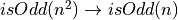 must be true after all.
We can now see the strategy of proof by contradiction as the application of a universal generalization. It’s just another valid inference rule. We can also see how we can apply it to specific cases to prove particular conjectures of interest. In the following example, for the sake of completeness, we first restate the law of the excluded middle and the proof that negation elimination is valid (relying on em). Next we formulate the so-called proof strategy of proof by contradiction and prove that it is valid with a one-line proof. What we see now in formal logic is that proof by contradiction involves first rewriting a goal into a new form, then asserts that if assuming that a given proposition is false leads to a contradiction, one can deduce that the proposition is true. The proof is by simple application of negation elimination. Finally, we prove that an equivalent rule is valid, and we prove it by applying our newly validated strategy of proof by contradiction.
axiom em : ∀ P : Prop, P ∨ ¬P

theorem neg_elim: ∀ P : Prop, ¬¬P → P :=
begin
  assume P : Prop,
  assume pfNotNotP : ¬¬P,
  cases em P,
    assumption,
    contradiction,
end

theorem proof_by_contradiction :
    ∀ P : Prop, (¬P → false) → P :=
        neg_elim

-- General strategy for PBC
namespace bycontradiction
axiom Q : Prop
example : Q :=
begin
  apply proof_by_contradiction,
  assume nq,
  sorry
end
end bycontradiction

-- If not P implies contra then P
example: ∀ P Q : Prop,
    (¬P → (Q ∧ ¬ Q)) → P :=
begin
  intros P Q,
  assume pfNotPImpliesQAndNotQ,
  apply proof_by_contradiction,
  assume pfNotP,
  have pfQAndNotQ := (pfNotPImpliesQAndNotQ pfNotP),
  show false, from (pfQAndNotQ.right pfQAndNotQ.left),
end
3.10.4.8. Proof By Contrapositive
If it’s true that if it is raining, then the streets are wet, then if the streets are not wet then it must not be raining:  . Similarly, if it’s true that if the streets are not wet then it’s not raining, then it must be true that if it’s raining the streets are wet:
  . The strategy of proof by contraposition relies on this second reasoning principle. If it’s valid, then to prove
  it suffices to prove
  . We now show that this strategy is valid in classical reasoning.
The theorem states that from a proof of the contrapositive of an implication, a proof of the implication itself can be constructed.
axiom no_contra : ∀ { P }, ¬(P ∧ ¬P)  -- we're proved this before
axiom neg_elim : ∀ (P : Prop), ¬ ¬ P → P

theorem proof_by_contraposition:
    ∀ P Q : Prop, (¬Q → ¬P) → (P → Q) :=
    begin
        intros P Q,
        assume nqnp p,
        have nqf : ¬Q → false, from
        begin
            assume nq,
            apply no_contra (and.intro p (nqnp nq))
        end,
        have nnq : ¬¬Q := nqf,
        show Q,
        apply neg_elim,
        assumption,
    end

-- the general approach
namespace bycontraposition
axioms (P Q : Prop)
#check nat
example : P → Q :=
begin
  apply proof_by_contraposition,
  assume nq,
  sorry
end

end bycontraposition

lemma zeqz' : 0 = 0 → true :=
begin
    apply proof_by_contraposition,
    assume nt : ¬true,
    have pff := nt true.intro,
    show ¬0 = 0,
    from false.elim pff
end

/-
Compare what by_contrapositive does to goal with what by_contradiction does to the goal.
-/

lemma zeqz'' : 0 = 0 → true :=
begin
  apply proof_by_contradiction (0 = 0 → true),
  sorry
end
EXERCISE: Does proof by negation require classical reasoning?
EXERCISE: Is proof by contradiction needed to prove that the square root of two is irrational, or will a proof by negation do?
3.10.4.9. DeMorgan’s Laws
We now turn to the question, how do and, or, not, and implies interact? In particular, we prove both of DeMorgan’s laws. These laws explain how negations distribute over disjunctions and conjunctions, respectively. The first states that 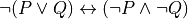 . That is, if it’s not the case that at least one of P or Q is true, then both P and Q are false. The second rule states that
 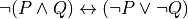 . That is, if it’s not true that P and Q is true, then at least one of P or Q is false.
Proving that the first law is valid in constructive logic is a homework problem. The second law law is not valid in constructive logic but is valid in classical logic, using the law of the excluded middle. Here we use Lean’s classical.em to enable classical reasoning.
axiom em: ∀(P: Prop), P ∨ ¬P

theorem Demorgan2 :
  ∀ P Q: Prop, ¬P ∨ ¬ Q ↔ ¬(P ∧ Q) :=
begin

  show ∀ P Q: Prop, ¬P ∨ ¬ Q ↔ ¬(P ∧ Q), from
  begin
  -- introduce assumptions of P and Q
  assume P Q,

  -- prove implication in each direction
  apply iff.intro,

  -- first, implication in forward direction
  show ¬P ∨ ¬Q → ¬(P ∧ Q), from
    begin
    -- goal is an implication
    -- so assume premise, and ...
    assume pf_np_or_nq,
    -- ... show conclusion
    show ¬(P ∧ Q), from
      begin
      -- remember ¬ is an implication in Lean
      -- so, assume premise, and ...
      assume pf_p_and_q,
      -- show conclusion
      show false, from begin
        -- by case analysis on ¬P ∨ ¬Q
        cases pf_np_or_nq with pf_np pf_nq,
        -- consider case where ¬P is true
          have pf_p := pf_p_and_q.left,
          exact pf_np pf_p,
        -- case where ¬Q is true
          have pf_q := pf_p_and_q.right,
          exact pf_nq pf_q,
        end
      end,
    end,

  -- now implication in reverse direction
    show ¬(P ∧ Q) → ¬P ∨ ¬Q, from
      begin
      -- assume premise
      assume pf_n_p_and_q,
      show ¬P ∨ ¬Q, from
        begin
        -- consider cases for P using em
        cases (em P) with pf_p pf_np,
          -- consider cases for Q using em
          cases em Q with pf_q pf_nq,
            -- P true, Q true
            have pf_p_and_q := and.intro pf_p pf_q,
            have pf_false := pf_n_p_and_q pf_p_and_q,
            exact false.elim pf_false,
            -- P true, Q false
            exact or.intro_right (¬P) pf_nq,
          -- P false
          exact or.intro_left (¬Q) pf_np,
      end,
    end,
  end,
end
3.10.4.10. is equivalent to  
In classical logic, if whenever P is true then so is Q, and if Q isn’t true, then P must not be. In constructive logic, this is not a valid rule. By limiting the possibilities for P to two cases, and insisting that one of them must hold, the law of the excluded middle makes this principle valid.
In the first half of the following proof, we include informal documentation and use a somewhat more verbose “show/from” style. In the second half, we leave out the commentary. A good way to construct natural language proofs, as you can see here, would be to comment a formal proof and then erase the formal part.
theorem altImplication:
  ∀ P Q: Prop, (P → Q) ↔ (¬P ∨ Q) :=
begin
  -- to show ∀ P Q: Prop, (P → Q) ↔ (¬P ∨ Q)
  -- we first introduce assumptions of P and Q
  assume P Q,
  -- next we prove implication in each direction
  apply iff.intro,
    -- first we prove forward direction
    -- we start by assuming the premise
    assume pf_p_imp_q,
    -- note that without em, we're stuck
    -- key is case analysis on P given em
    cases (em P) with pf_p pf_np,
      -- case where P is true
      -- construct a proof of Q
      have pf_q := (pf_p_imp_q pf_p),
      -- then prove goal by or intro
      --exact or.intro_right (¬P) pf_q,
      exact or.inr pf_q, -- shorthand!
      -- case where ¬ P is true is easy
      exact or.inl pf_np, -- shorthand

    -- prove implication reverse direction
    assume pf_np_or_q,
    assume pf_p,
    cases pf_np_or_q with pf_np pf_q,
      have pf_false := (pf_np pf_p),
      exact false.elim pf_false,
      assumption,
end
Next we prove that a bi-implication is equivalent to the proposition that either both sides are true or both sides are false.
theorem altEquivalence :
∀ { P Q : Prop }, (P ↔ Q) ↔ ((P ∧ Q) ∨ (¬P ∧ ¬Q))
:=
begin
  assume P Q,
  apply iff.intro,

    intros,
    have pq := iff.elim_left a,
    have qp := iff.elim_right a,
    cases (em P) with p np,
      cases (em Q) with q nq,
        exact or.inl (and.intro p q),
        exact false.elim (nq (pq p)),

      cases (em Q) with q nq,
        exact false.elim (np (qp q)),
        exact or.inr (and.intro np nq),

    intros,
    cases a,
      apply iff.intro,
        intro,
        exact a.2,

        intro,
        exact a.1,

      apply iff.intro,
        intro,
        exact (false.elim (a.1 a_1)),

        intro,
        exact (false.elim (a.2 a_1)),
end
3.10.5. Backwards Reasoning
This chapter has covered negation and numerous proof strategies involving negation, including proof by negation, contradiction, and contraposition; modus tollens; disjunctive syllogism; and so forth. We’ve seen that each of these strategies involves nothing more than the application of a valid rule of reasoning (sometimes constructive, sometimes classical).
The best way, in our view, to think about what applying a proof rule does is to construct a proof, albeit sometimes ones with some remaining holes to be filled. The holes then become sub-goals, and once they are taken care of the overall proof term, in which the selected rule is applied to arguments that have now been provided, is complete.
There is a different way to think about what’s happening here. The phrase you will hear is backwards reasoning. Suppose we already have a proof, pq, of some proposition, , and that we are in a situation where we need a proof of Q (to provide such a proof is our goal). It would of course suffice to provide such a term by applying pq, our proof of , to some argument of type P. A term-style proof of Q could thus be written as (pq _), where the hole will be filled in with some value/proof of type P. In a tactic-style proof, one would write (apply pq _), or, more likely, just apply pq, letting Lean determne that there’s a remaining argument to be provided, i.e., hole to be filled, i.e., meta-variable to be assigned a value.
In any case, the goal of providing a proof of Q has been reduced, by the application of a proof of , to the goal of providing a proof of P. We have in a sense transformed and simplified the goal of producing a proof of Q by moving backwards through a proof of , thus reducing the goal to one of providing an argument (a proof) of type P. One continues in the so-called backwards style until all holes have been filled.
We prefer to view this process as one of top-down refinement, in which one provides the overall proof term at the start of the process, albeit with holes, and where then one iteratively and incrementally refines the holes in a type-guided style until all terms have been completed and no holes remain.
That said, the backwards reasoning viewpoint commonly taken and is also helpful. Consider what we mean, for example, when we say informally that we will apply a proof by contradiction strategy to prove some conjecture, P. What we are really doing is giving the final proof in the form of the application of a proof of the validity of double-negation elimination to a proof of , where that proof remains to be developed. The goal of proving P is thus reduced to the goal of producing a proof of . One then constructs this argument as a sub-goal. The final proof term is an application of the given inference rule to the argument.
Let’s say it in different words. To prove P it suffices to apply negation elimination to a proof of . If the current goal is P, then a command to apply negation elimination, without giving the argument that this function (and it is a function!) takes, is in effect saying that my final proof is neg_elim _, where the underscore needs to be filled in with a proof of . Constructing that proof becomes the new sub-goal. The original goal is thus reduced to the goal of filling the hole. Once again it appears in a way that we are reasoning backwards, from our initial goal to goals that are ever closer to disappearing entirely, which is exactly what happens when there are no more holes to fill in the overall proof term we are constructing.
3.10.6. Natural Language
The proof strategies we have covered in this chapter are used widely in mathematics, logic, and computer science. Any mathematically educated person knows them and has a good sense for when to apply them. They are usually invoked in natural language proofs, rather than in formal proofs. Having studied the formalism shows exactly how they work.
An informal proof typically begins with a brief declaration of the strategy to be used. One explains that to prove the original goal, it will suffice to prove the goal as transformed by the application of the reasoning principle; for then the reasoning principle can be applied to that result to obtain a proof of the original conjecture. Having obtained proof of the transformed goal, or sub-goal, one finally reminds the reader that, in combination with the application of the reasoning principle, it suffices to established a proof of the original goal.
Here’s an example. Suppose that the original goal (conjecture to be proved) is some proposition, P and that the selected strategy is a proof by contradiction. An informal proof could be written as follows. “We are to prove P. We will prove it using the strategy of proof by contradiction. We will thus assume not P and show that this leads to a contradiction. This will show that not P is false, and thus that not not P is true. By applying the rule of negation elimination we deduce that P must be true.” When speaking to a mathematically mature audience, one can be brief in explaining the use of such proof strategies, as mathematically mature readers are already familiar with the ideas.
Most mathematicians, logicians, and computer scientists assume the axiom of the excluded middle. Only in cases where there are concerns about whether proofs are constructive or not does one need to remind the reader that one is employing classical reasoning. Such cases do arise in computer science, especially in the areas of programming languages and the production of formally verified, e.g., provably secure, code.
3.11. Exists
In an earlier chapter, we learned how to state and prove claims asserting that some proposition is true for all objects of some type. We express such claims as universal generalizations. The proposition in question is usually formed by applying some predicate to any object of the given type. The overall formula in question is usually of the form, , where P is a predicate that is then applied to t, where t can be bound to any value of type T. The overall proposition will be true if P t is true for every possible value of t.
Sometimes, we want to make a related but distinct claim: not that some proposition is true for every object of some type, but only that there is some object (at least one) of the given type for which a proposition is true. To do this, we use an existentially quantified proposition.
For example, we might want to assert that there exists some natural number that is prime; or there exists at least one ball that is blue; or there is someone who is happy. We often want to assert that there exists some object of a given type having some property (being prime, blue, or happy, for example), where that property is expressed as a predicate. And once, again, to do this, we use an existentially quantified proposition.
In this chapter, we explain the form of such a propositions, its related introduction and elimination rules, how these rules enforce the intended meaning of such propositions, and how to use these rules. We will see how to construct proofs of existence in Lean, and what one can deduce from proofs of existentially quantified propositions.
3.11.1. Formula
An existentially quantified proposition asserts that there is some value of a specified type that makes a corresponding proposition true. The typical form of such a proposition is 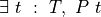 . The backwards E is the existential quantifier of predicate and constructive logic; t is an identifier that is intended to be bound to some value of the type, T, and it is meant to be bound to an object of this type that makes the predicate, P, applied to t, true.
3.11.2. Interpretation
We interpret an existentially quantified formula as asserting that some object of the specified type exists that makes a specified proposition true.
As a reminder, recall that a predicate,  , can be read as formalizing a property, P of objects of type T. For example, a predicate,
  , could be read as formally representing the property of a person being from Charlottesville. When applied to any object, p, of type Person, this predicate would yield a proposition. Some people are from Cville; some aren’t; and this predicate formally represents the real-world property of being from Charlottesville if the proposition it returns for any given person, p, is true if and only if (the real-world person represented by the logical term) p really is from Charlottesville.
Given this reading of predicates, we can now see that it makes sense to pronounce the proposition, , as there is some (at least one) t, of type T, with property P. This is how we encourage you to pronounce and understand what an existentially quantified proposition asserts.
Consider a simple arithmetic example. The claim that there is some natural number, m, such that m + m = 8 can be formalized as an existentially quantified proposition. We can write this claim formally as:math:existsm:nat,m + m = 8. We would pronounce this proposition as, “There is some natural number m such that m + m = 8.” Before the comma, the identifier, m, of type, nat, is introduced, and after the comma m is constrained to be a value that satisfies the predicate, m + m = 8 (which given any particular value of m yields a proposition that might or might not be true. If there is some (at least one) value for m that satisfies the predicate, then we judge the existentially quantified proposition to be true, and otherwise to be false. In this case there is a value for m that satisfies the predicate. It is found by simple algebra to be m = 4.
We use the term, witness, to refer to a value that makes an existentially quantified proposition true. Here, we have a witness, m = 4. We can easily construct a proof that letting m = 4 makes, m + m = 8, true. The proof is by reduction of the expression, m + m to 8 and the reflexive property of equality: in Lean, eq.refl 8. So what we have then, as indisputable evidence that the existentially quantified proposition is true is a withness and a proof, a pair, where the proof show that that specific witness makes the given proposition true. This observation takes us directly to the introduction rule for existentially quantified propositions.
3.11.3. Introduction
In constructive logic, a proof of an existentially quantified formula is pair: a witness, m, and a proof that the corresponding proposition is true for that particular witness. A proof of an existentially quantified proposition is thus a pair, <w : T, p : P>, where w is a witness and p is a proof that P is true for that witness. In the typical case, P will be a predicate, and the corresponding proposition will be obtained by applying P to t, so the pair will be of the form, <w : T, p : P t>.
In constructive logic such a pair is called a dependent pair, because the type of the second value in the pair, p, depends on the value of the first element in the pair, w. To see this, just recall that in constructive logic, propositions are types; and different propositions are different types. Now consider a predicate, isEven, for example, over the natural numbers. The proposition, isEven 2 is one type, while isEven 4 is a different type. Each of these types has its own set of values, which are the proofs of the respective propositions. Now it is easy to see that there are many different proofs that there exists an even number. One could take the form of a pair with the value 2 and a proof of isEven 2; another could be a pair with first element, 4, and a proof of isEven 4 as a second element. In the first case, the second element of the pair is a value (a proof) of the type isEven 2, while in the second case the proof is a value of type isEven 4. In each case, the type of the second element depends on the value (of type nat) of the first element.
The concept of dependent pairs is at the heart of the introduction rule for existential propositions. To construct a proof of  one must exhibit a specific pair of values: the first, a value, w, short for witness, of type T; the second, a value of type P w, namely a proof that the specific proposition, P w, for that particular witness, is true. You should stop now and think about why the existence of such a pair proves that there really is an object of the specified type with the specified property.
Here, then, is the formal introduction rule for exists. It just states precisely what we’ve just said. If you know that T is any type, P is a predicate on objects of that type, w is a specific value (witness) of that type, and p is a proof that w satisfies P, then you can validly deduce  . The first two arguments to this proof constructing rule are implicit, which means that in practice, one need only given w and a proof of P w as explicit arguments.

Here’s an example in Lean, formally proving that there is an m of type nat such that m + m = 8. We give the proof in both term- and tactic-script style. We give an exact (complete) proof term in the first case, with both arguments provided. Next we give the same term-style proof but using Lean’s convenient angle bracket notation as a shorthand for the application or exists.intro. Lean knows by the goal to be proven to interpret this notation not as a shorthand for and.intro (which we saw earlier) but as a shorthand for exists.intro. This notation makes it clear that a proof of a existentially quantified proposition is essentially a dependent pair, comprising a witness and a proof of a proposition about that witness. In the third, tactic-style, case, we apply exists.intro only to its first argument (a witness that we believe makes the predicate true), leaving the construction of the proof as a subgoal. In practice, such a tactic-style proof is what one would ordinarily encounter or use, except for simple cases.
example : exists m, m + m = 8 :=
    exists.intro 4 (eq.refl 8)

example : exists m, m + m = 8 :=
    ⟨ 4, eq.refl 8 ⟩

example : exists m, m + m = 8 :=
begin
  apply exists.intro 4,
  exact eq.refl 8
end
EXERCISE: Formally state and prove the existentially quantified proposition that there exists a natural number, m, such that m squared is 25. Use a lambda expression to formalize the predicate after the comma in your expression.
What follow are some examples that illustrate the use of exists.intro. The first example defines a function that takes exactly the arguments needed to apply exists.intro, an it then applies it.
def existsIntro (T: Type) (P: T → Prop) (w : T) (pw : P w) :
  exists w, P w :=
exists.intro w pw

#check existsIntro
This next example does essentially the same thing as the preceding example, except it uses axioms instead of arguments to introduce the assumptions that we’re given the “ingredients” needed to apply exists.intro. It then applies this rule using term-style presentations, the second of which uses the angle bracket shorthand.
variable T : Type
variable witness : T
variable predicate : T → Prop
variable proof : predicate witness

-- direct use of exists.intro
example : ∃ m, predicate m :=
    exists.intro witness proof

-- shorthand
example : ∃ m, predicate m :=
    ⟨ witness, proof ⟩

#reduce fourAgain
The next example shows how we can use an existentially quantified proposition to define the property of a natural number being even. We then use this definition to state the proposition that 10 is even, which we then prove using the exists.intro proof rule. In the proof script, we introduce a new tactic, unfold. It simply replaces a term, here isEven, with its definition. It’s not strictly necessary in this case, as the proof would “go through” without it, but it does make it clear that what has to be proved is an existentially quantified proposition. Study how the tactic state changes as you move through the steps of this proof script in Lean. Note in particular how the application of exists.intro to the witness, 5, causes the predicate to be replaced by the proposition obtained by applying the predicate to the witness. The resulting proposition is what has to be proved to show that that specific witness has the property that is claimed, here of being even.
def isEven (n : nat) : Prop :=
    ∃ m, 2 * m = n

example : isEven 10 :=
begin
  unfold isEven,
  apply exists.intro 5,
  apply rfl,
end
3.11.3.1. Understand Your Tools
Lean comes with libraries that define all of the data types that we’ve been using, including nat, and including many operations on values of these types. For example, Lean defines operators for multiplying and dividing nat values. One has to be exceptionally careful to understand exactly how these operations behave. For example, what, in Lean, is the result of dividing the natural number, 7 by the natural number 3, yielding a natural number? If you’re inclined to answer, 7/2, that’s wrong because that’s a rational number, not a natural number. The answer is 2, because 2 is the natural number quotient of 7 / 2. The remainder is 1. When it comes to computer arithmetic, one must be exceptionally careful to understand precisely how the various operators work, because they do not necessarily do what your well developed intuition might suggest.
def n := 7 / 3
#eval n
Even more confusingly, Lean’s libraries, which are implicitly imported when Lean starts to run, also define, and sometimes implicitly apply, methods for converting objects of one type into another. Sometimes this is convenient. Sometimes it is annoyingly misleading. Here’s an example of the latter in which it appears that Lean is accepting 3.5 as a value of type nat. What it’s actually instead is implicitly applying a type conversion operator to convert 3.5 into 3. The #eval line makes it clear that n is bound to the nat value, 3, not to 3.5.
def n : nat := 3.5
#eval n
We can now put these two facts together to construct two “proofs” that seem just wrong. To begin, we formalize the predicate, isEvenBad, as described above. The first example then “proves” that 7 is even using 3 as a witness. Can you already see why this is going to work? The second example proves that 7 is even using 3.5 as a witness, even though the type of value expected is nat. Do you now see why this will work?
def isEvenBad (n : nat) : Prop :=
    exists m : nat, n / m = 2

example : isEvenBad 7 :=
    ⟨ 3, rfl ⟩

example : isEvenBad 7 :=
    ⟨ 3.5, rfl ⟩
Clearly we haven’t actually proven that 7 is even. It’s not. Rather, our definition of isEvenBad is subtly flawed. We mistakenly assumed that we were working in the real numbers, in which case it’d be perfectly good, as 7/3 would then definitely not be equal to 2. But when working in the natural numbers, 7/3 really is defined to be 2 (remainder 1). It’s our definition of evenness that is wrong. In the second example, Lean is implicitly converting 3.5 to 3 so that it becomes an argument of the right type. It does this in order to be “helpful” to us; but doing so, combined with the fact that we’re working in the natural numbers, makes it look like we’ve proved an absurdity: that 7 is even, using a witness that isn’t even of the required type. Care must be taken even when using a nearly infallible proof assistant. The problem isn’t really with the tool, it’s that one must understand one’s tools thoroughly in order to use them with justified confidence.
3.11.3.2. Example : There exists a non-zero natural number
We now assert and give you several proofs of the proposition that there exists some natural number that is not equal to zero. The proposition is of course true. A formal proof of it will be a pair, <n, p>, where n is a natural number that is not 0, and p is a proof that that particular number is not equal to zero. We use this example to further discuss the use of the cases tactic applied to proofs of equalities, and then to introduce a bit of Lean automation, namely the dec_trivial tactic. We won’t try to explain how it works, but we will alert you to it so that you can use it in the future.
Our first proof, in the following block of logic, applies exists.intro to a witness. The remaining proposition to be proved is a negation. A negation is an implication, so we assume the premise, at which point the only thing we need is a proof of false. The key idea is that from a proof of 0 = 1 a proof of false can be constructed. One looks at each of the ways in which such a proof could have been constructed, and for each, one must show that a proof of false can be derived. That is, one uses case analysis on the possible constructors of a proof of 0 = 1. The only constructor of a proof of an equality is eq.refl; but eq.refl cannot possibly have constructed such a proof, as it takes only one value, t, and can only return proofs of the form, t = t. There are no other cases to consider, so for each constructor that could have been used to construct the proof of which there there are none, a proof of false can be derived, so the goal can be considered to be proved.
example : exists n : nat, 0 ≠ n :=
begin
  apply exists.intro 1,
  assume h,
  cases h,
end
The next two examples give essentially the same proof. What they are intended to teach you is that you can use tactic-style proofs within term-style proofs. This is important if you want to write a term-style proof of our simple proposition, because you don’t yet know what term-style constructs to use where cases appears in the tactic script. Rather than explain that somewhat more complex issue at this point, we show you how to revert to tactic-style proving in the middle of a term-style proof. The key is that, where you need a term, you can use the keyword by followed by a tactic style proof script! As the second example here shows, you don’t have to use a begin-end pair. It is however often useful to do so.
example : exists n : nat, 0 ≠ n :=
  exists.intro
    1                   -- witness
    (λ h : (0 = 1),    -- proof of negation
      by begin
          cases h
        end
    )

example : exists n : nat, 0 ≠ n :=
  exists.intro
    1
    (λ h : (0 = 1),
      by cases h)
Our second proof introduces the use of the dec_trivial tactic in Lean. This tactic can be used to prove simple decidable propositions. A proposition is said to be decidable if it can be shown to be essentially the same as the proposition, true, or the proposition, false. The key idea here, without getting into details, is that the proposition, 0 = 1, is decidable; the dec_trivial tactic can also find a way to show it; it can then use that method to decide that the proposition is essentially the same as false. That’s all there is to it. When you’re faced with the need to prove some arithmetic proposition, try dec_trivial. Our final example combines the use of dec_trivial with Lean angle-bracket notation to give a beautifully concise proof of our existentially quantified proposition.
example : exists n : nat, 0 ≠ n :=
begin
  apply exists.intro 1,
  assume h,
  dec_trivial,
end

example : exists n : nat, 0 ≠ n :=
    ⟨ 3, dec_trivial ⟩
EXERCISE: Suppose P is some predicate of type  . Could you ever prove,
  ? Why or why not?
EXERCISE: Suppose P is any predicate of type . Can you prove,  ? Explain.
EXERCISE: Prove  .
.
EXERCISE: Compare and contrast the answers and the underlying concepts underlying the previous three exercises.
3.11.4. Elimination
The elimination rule for existentially quantified formulas gives you a way to use a proof of such a proposition. The statement of the elimination rule is a bit complicated but the idea is really very simple: if you have a proof of , then you know there is some object, amongst all the values of type T, that has property P, and so you can give a name to it! That is the key idea: give a name to the object that you know exists. Let’s call it w (for witness). Now, because this w was picked to be a object with property P, you can assume that you also have a proof of P w.
From a proof of an existentially quantified formula, you can obtain a witness and a proof that that witness has the specified property. You can then use that witness and that proof in constructing a proof that you might need.
3.11.4.1. Example: If there’s a green ball, there’s a ball
What follows is a simple example. We prove a proposition that, when translated into English, asserts that if there is a green ball, then there is a ball. More precisely, for any type, Ball, and for any predicate, isGreen, concerning balls (objects of type Ball), then if there is a ball, g, with the property, isGreen, then there is a ball, b. Any object of any type makes the proposition, true, true, because it is already and always true. So all that the conclusion really asserts is that there is at least one ball. In particular, if there is a green ball, we can simply point to it as a witness to the proposition that there is some ball.
example :
  ∀ (Ball : Type),
      ∀ isGreen : Ball → Prop,
          (exists (g : Ball), isGreen g) →
              ∃ b : Ball, true :=
begin
  intros Ball isGreen,
  assume h,
  apply exists.elim h,
  assume w,
  assume Gw,
  apply exists.intro w,
  trivial,
end
The first line of the proof applies forall introduction by assuming that we are given a specific type, Ball, and a specific predicate, isGreen, with balls as arguments. What’s left to prove is an implication: one that asserts that if there is a green ball, then there is a ball. To prove this implication, we assume its premise to be true (that there exists a green ball). We give the name h to an assumed proof of this premise.
We now have a proof of an existentially quantified proposition, h, in our context, with a second existentially quantified proposition left to prove. To prove the remaining goal, we will need a witness along with a proof of true. The latter is easy: true.intro will do. But from where will we get a witness?
The answer is by applying the exists elimination rule to h. Having accepted that there is a green ball, the exists elimination rule lets us give it a name. That object will then be the witness we need to apply the exists introduction rule to finish off the proof. In the next line of the proof we thus apply the exists.elim rule to the proof, h.
The immediate result is that the remaining goal is transformed from  into a more complex goal:
  . It says that for any ball, a, if a is green, then there is a ball. The lambda expression is simply our predicate, isGreen.
To prove this universal generalization, we assume that we have an object, a, of type Ball. Ah ha! That’s how we get a named ball. Then to prove the remaining implication, we assume the premise, that that ball is green. Ah ah, again! That’s how we get a proof that our witness is green.
In this case, we don’t really need this proof of greenness, as all we have to show is that there is some ball. The rest of the proof is simply by applying exists.intro to the witness for which we now have a name, and to a proof of true, which is simply true.intro.
3.11.4.2. The cases tactic
The elimination rule for an existentially quantified proposition is, in spirit, like the elimination rules for conjunction: it provides you with access to the elements from which a proof was constructed. In the case of a conjunction, the elements of a proof are proofs of the left and right conjuncts. For a proof of an existentially quantified proposition, the elements are a witness and a proof that it has the given property. The elimination rules in each case provide access to these elements.
The cases tactic can be employed to good effect here. As we have said previously, what it does is to analyze each way in which a given proof could have been constructed, and it presents each case separately, with names and types given to the arguments to which an introduction rule must have been applied to construct the given proof.
We’ve already seen several examples of this idea. When we apply the cases tactic to an assumed proof of an impossible equality, such as 0 = 1, it finishes off the proof, because it determines that there are no cases to consider: no way that eq.refl could have been used to create that proof.
When we apply the cases tactic to a proof of a disjunction, by contrast, we end up with two cases to consider. One possibility (one case) is that the proof was constructed by or.inl applied to a proof of the left disjunct. The other possible case is that the proof was constructed by or.inr applied to a proof of the right disjunct. In each case, either Lean gives, or we provide, a name for the argument that must have been given to the constructor as an argument.
Although we haven’t yet seen cases applied to a proof of a conjunction, it makes sense now that it should work. We’d expect it to determine that there is only one case: and.intro was applied to two proofs, one of each conjunct. Cases then should give these proofs names and types so that we can use them. In fact that is just what it does. Here’s a simple example.
example : ∀ (P Q : Prop), P ∧ Q → P :=
begin
  intros P Q,
  assume h,
  cases h with p q,
    exact p,
end
Now finally we come to the cases tactic applied to a proof of an existentially quantified proposition. It does what one might now suspect. It gives names and types for a witness and a proof to which exists.intro must have been applied to construct the given proof. The cases tactic thus provides a nice shorthand way to deal with a proof of an existentially quantified proposition.
example :
  ∀ (Ball : Type),
  ∀ (isGreen : Ball → Prop),
  (∃ (g : Ball), isGreen g) →
  ∃ b : Ball, true :=
begin
  intros Ball Green,
  assume h,
  cases h with w Gw,
    apply exists.intro w,
    exact true.intro,
end
The cases tactic is the easiest way to use a proof of an existentially quantified proposition. It replaces the proof with a witness and proof that that witness has the specified property. These objects can then be used in proving the remaining goal to be proved.
Example: If n is a multiple of 4 then n is even.
In this example, we restate a good definition of what it means for a natural number, n, to be even: there exists some m such that n = 2m. Then using this definition, we assert, and then prove, that if any number, n, is a multiple of four, then n is even.
This example has an existentially quantified propositions as a premise and the conclusion of an implication. We will have to use both elimination and introduction rules for exists to complete the proof. The key insight seen in the proof is the choice of a witness. Before you go any further, if you’re given a number, n, that is a multiple of 4, which is to say that there is a witness, w such that n = 4*w, then what witness can be used to prove that n is even?
The proof also uses a proof, already provided in Lean’s libraries, of the associativity of multiplication. You should recall that function application is left associative, so an expression, a * b * c, is understood to mean (a * b) * c. If you mean a * (b * c), you must use explicit parentheses. Operators, such as *, are in general not associative, so Lean won’t just assume that a * b * c = (a * b) * c. If * means subtraction, for example, then it’d be wrong to assume these terms are always equal. If you want to rewrite a term, such as a * b * c, into another term, such as c = (a * b) * c, you have to have a proof that it’s valid to do so. The proof, nat.mul_assoc, is such a proof. If you were writing a natural language proof you could say we rewrite the first expression into the second using the associativity of multiplication.
We can use #check to see the exact proposition that has been proved in Lean. See the following code block. Be sure you understand where parentheses go if they’re not explicit. Remember, function application is left associative, so an expression such as a * b * c means (a * b) * c. If you want a * (b * c), parentheses must be used.
#check nat.mul_assoc
So now here is our main example.
-- An evenness predicate using exists
def isEven (n : nat) : Prop :=
    ∃ m, 2 * m = n


-- For any n, if n is a multiple of 4 then n is even
example : ∀ n : ℕ, (∃ m, n = 4 * m) → isEven n :=
begin
  intro n,
  assume h,
  cases h with w pf_w,        -- elimination rule
    unfold isEven,
    apply exists.intro (2 * w), -- smart choice of witness!
    rewrite pf_w,
    rewrite<-nat.mul_assoc,     -- library: mul is associative
    apply rfl,
end
This proof uses a theorem for which a proof is provided by Lean’s standard library: that natural number multiplication is associative. Practical use of a theorem prover such as Lean requires deep familiarity with the contents of the libraries To learn Lean’s libraries is beyond the scope of this course. But once you are done with this course, you will be in a good position to learn them should you wish to.
Example: If there is a natural number has properties P and Q, then there is one that has property P. Note that in this formulation, we take P to be a predicate and Q to be a predicate over natural numbers. We then use the predicate  to express the property of having both properties, P and Q.
theorem forgetAProperty :
    forall (P Q : ℕ → Prop), (∃ n, P n ∧ Q n) → ∃ n, P n :=
begin
  intros P Q,
  assume h,
  cases h with n pq,
    cases pq with Pn Qn,
      exact exists.intro n Pn,
end
EXERCISE: Prove: Prove that if there exists a natural number, n, that satisfies the predicate, P n and S n, then there exists a natural number that satisfies the predicate S n and P n (in that reversed order).
Todo
Give actual exists.elim inference rule.
3.11.5. Expressing Subtle Ideas with Mixed Quantifiers
The ideas that we’ve expressed in logic up until now have been pretty simple. Now that we’re equipped with both universal and existential quantification, and given that we can use these quantifiers together in various ways, we can express more interesting and subtle ideas. Here, for example, is how we might formalize and then even prove the claim that if there is a person (someone) who can be fooled at any time, then at any time someone can be fooled.
example:
    ∀ (Person Time : Type),
    ∀ (Fool : Person → Time → Prop),
    (∃ p : Person, ∀ t : Time, Fool p t) →
    (∀ t : Time, ∃ p : Person, Fool p t) :=
begin
  intros Person Time Fool,
  assume someoneAllTime,
  intro time,
  cases someoneAllTime with person fool,
    apply exists.intro person,
    exact fool time,
end
EXERCISE. To discuss. Does this claim make sense? Why? Who is the witness in the proof of the conclusion of the implication? Give a clear English language explanation of why the proposition logically makes sense.
The identifiers we used in the preceding example suggest that we are speaking about a domain of people, time, and fools. Without changing the logic at all, we can replace these identifiers with others that have no domain-specific connotations. We end up with a nice general result, or theorem. It might be read as saying, if every object of some kind has some particular property at every point in time, then at every point in time some object of that kind has that property.
example:
    ∀ (S T : Type),
    ∀ (P : S → T → Prop),
    (∃ s : S, ∀ t : T, P s t) →
    (∀ t : T, ∃ s : S, P s t) :=
begin
  intros S T P,
  assume PsomeSallT,
  intro t,
  cases PsomeSallT with s allTPst,
    apply exists.intro s,
    exact allTPst t,
end
EXERCISE: Is the converse proposition true? First, state the converse in English. Second, explain why it is or isn’t a valid principle. If you claim it is, give a proof. If you claim it isn’t, give a compelling explanation. Extra credit for proving it in this case.
EXERCISES: Practice translating English statements into logic by filling in the missing logic in the following code block.
axioms (Person Time : Type) (Fool : Person → Time → Prop)

-- Everyone can be fooled sometimes
def p1 : _ :=
sorry

-- There's a time when everyone can be fooled at once
def p2 : _ :=
sorry

/-
If there's a time when everyone can be fooled, then anyone
can be fooled sometime
-/
def p3 : _ :=
sorry

-- There's someone who can always be fooled
def p4 : _ :=
sorry

-- At any time someone can be fooled
def p5 : _ :=
sorry

/-
If there's someone who can be fooled anytime, then
at any time, someone can be fooled
-/
def p6 : _ :=
sorry
3.11.5.1. Negating Existential and Universal Quantifiers
We can express even more interesting ideas with combinations of negations with universal and existential quantification. Here are formalizations of various propositions illustrating this point.
This example also introduces a new (to us) construct in Lean: sections. A section is used when we want to declare identiers once that are then assumed to be included in each of the following definitions in a file.
section ucantfoolme

variables (Person Time : Type) (Fool : Person → Time → Prop)

-- There's no time when you can fool me
example : ∃ (me: Person), ¬∃ t : Time, Fool me t := sorry

-- at any time, you can't fool me
example : ∃ me : Person, ∀ t : Time, ¬Fool me t := sorry

-- Are these propositions equivalent?

-- How about these propositions?

--you cannot fool me all of the time
example : ∃ me : Person, ¬(∀ t : Time, Fool me t) := sorry

-- there exists a time when you cannot fool me
example : ∃ me : Person,  ∃ t : Time,  ¬Fool me t := sorry

end ucantfoolme
Is it true that if there’s not a time at which something happens, then at all times nothing happens, and vice versa?
example:
    ∀ (T: Type) (P: T → Prop),
    (¬(∃(t: T), P(t))) ↔
        ∀(t: T), ¬P(t) :=
begin
    assume T P,
    apply iff.intro,

    -- forward
    assume pf_not_exists_t,
    assume t,
    assume P_t,
    have ex_t := exists.intro t P_t,
    contradiction,

    -- reverse
    assume all_not_P,
    assume ex_t_P,
    cases ex_t_P with w Pw,
    have not_P_t := all_not_P w,
    contradiction,
end
Is it true that if something doesn’t happen all the time, then there is a specific time at which it doesn’t happen?
open classical

example :
    ∀ (T: Type) (P: T → Prop),
    (¬(∀ t: T, P(t))) ↔
        ∃ t: T, ¬P(t) :=
begin
intros,
apply iff.intro,

-- forward
assume not_all_t,

-- classical case analysis on (em (∃ (t : T), ¬P t))!
cases (em (∃ (t : T), ¬P t)) with ex_not_t not_ex_not_t,

-- case, it's true
exact ex_not_t,

-- case, it's not true
-- construct local proof of (∀ t, ¬ ¬ P t)
have contra_double_neg: ∀(t: T), ¬¬P t,
assume t,
assume n_P_t,
have ex_t := exists.intro t n_P_t,
contradiction,

-- construct local proof of (∀ t, P t)
have contra: ∀(t: T), P t,
assume t,
have nn_P_t := (contra_double_neg t),
cases em (P t) with P_t n_P_t,
    assumption,
    exact false.elim (nn_P_t n_P_t),

-- contradiction; QED case, QED forward
exact false.elim (not_all_t contra),

-- now for the backward direction
assume ex_not_t,
assume pf_all_t,
cases ex_not_t with w Pw,
show false, from
    begin
    have P_w := pf_all_t w,
    contradiction,
    end,
end
3.11.5.2. Extended Example: A Preview of Satisfiability
The simplest logic that we will discuss in this course is called propositional logic. It is a logic in which logical variables take the place of the propositions of predicate logic. A variable in turn is interpreted as having simple Boolean truth values. Propositional logic is the logic underlying the Boolean expressions found in the conditions of if and while statements. In fact, propositional logic is isomorphic to Boolean algebra.
Sentences in this logic thus include the following, where the letters are logical variables: P, P and Q, P and not P, and so forth. But now we consider each variable to have one of the two Boolean values.
A vitally important problem in propositional logic is to find values for the variables in a given sentence such that that sentence, when evaluated, reduces to the true Boolean value. For example, if the sentence is just, P, then by setting the value of P to the Boolean value, true, we make the sentence, P, true. If the sentence is P or Q, we can make it true by setting either or both of P and Q to true.
On the other hand, if the sentence is P and not P then neither of the two possible values of P will make the sentence true. If we set P to be true, then the sentence reduces to true and false, and if we set P to false, then the sentence is false and true. We note that proposition logical is classical, so the law of the excluded middle always holds: there really are only two possible values for any given proposition.
Many fundamental problems in computer science can be solved by algorithms that find values for all of the logical variables in a given sentence in propositional logic. While the problems we have looked at here involve only a few variables, in some cases one wishes to solve problems of this kind involving many, many thousands of variables, or even more.
The problem of finding satisfying solutions to expressions in propositional logic is knowns as the SAT problem in computer science, short for satisfiability. We discuss the importance and the nature of this problem further in the forthcoming chapter on formal languages, in which we formalize the syntax and semantics of propositional logic.
In the remainder of this chapter, we give a brief preview of the SAT problem using the tools we already have. The most important of these tools for our purposes here are as follows. First, in the higher-order logic of Lean, we can quantify over propositions. That is, we can write propositions that start with forall P of type Prop or with exists P of type Prop. We have seen many examples using forall. In this section, we see examples using exists P of type Prop.
When a proposition in predicate logic starts with exists, it sets up what you can think of as a search problem. To prove it, you have to search for and find a value that makes the following predicate true. All of the problems in this section, start with exists P of type Prop. This quantified expressions is then followed by a predicate, such as P and not P, for example. Your task is to give a witness for P that makes the following predicate true. If you can do this, then you have proved that the predicate is satisfiable. A value for P, in each of these problems, is itself a proposition! And to solve these problems, it will suffice to use only the propositions, true and false for these values.
What we’re doing here, then, is sort of simulating a much simpler propositional logic using the richer logic of Lean. Here’s a first example.
example : ∃(P : Prop), P :=
begin
  apply exists.intro true,
  exact true.intro,
end
The challenge here is to give a witness for P that makes the predicate, here just P itself, true. The proposition to be proved is that there exists such a proposition, P. Here we prove it by giving the proposition, true (not a Boolean value in Lean, mind you) as a value for P, i.e., as a witness. The resulting proposition to be proved is then just true, and that is trivially provable.
The next example seeks a value for P that makes the proposition, not P, true. Now, the value, false for P is a a satisfying solution.
example : ∃(P : Prop), ¬P :=
begin
  apply exists.intro false,
  assume f,
  contradiction,
end
Satisfiability problem can and generally do involve multiple logical variables. Here’s a problem where you have to “assign truth values” to two variables, P and Q in an attempt to make the sentence, P and Q evaluate to true. Taking the proposition, true, as a witness for both P and Q yields a satisfying solution, we the following proof certifies.
example : ∃(P Q : Prop), P ∧ Q :=
begin
  apply exists.intro true,
  apply exists.intro true,
  apply and.intro true.intro true.intro,
end
The expressions for which satisfying solutions are sought generally include negated as well as non-negated variables. Here we seek a satisfying solution for P and not Q. Setting P to be true and Q to be false makes the overall expression true. The resulting sentence is true and (not false). This reduces to true and true. And this is easily proved.
example : ∃(P Q : Prop), P ∧ ¬Q :=
begin
  apply exists.intro true,
  apply exists.intro false,
  apply and.intro true.intro,
  assume f, contradiction,
end
The sentences for which satisfying solutions are sought generally involve any of the usual Boolean connectives. Here’s an example that uses or. It is easy to see that there are two satisfying solutions for this problem: if P is set to true, then the sentence reduces to true or false, which is true; otherwise, if P is set to false, the sentence evaluates to false or (not false), which reduces to false or true, which is true, as proved here.
example : ∃(P: Prop), P ∨ ¬P :=
begin
  apply exists.intro true,
  left, -- short for apply or.inl
  trivial,
end
A sentence that is true for all every possible assignment of truth values to its variables is said to be logically valid. To complete a proof that P or not P is valid, we simply show that it is true for the only other possible assignment of a value, namely false to P.
example : ∃(P: Prop), P ∨ ¬P :=
begin
  apply exists.intro false,
  right, -- short for apply or.inr
  assume f,
  contradiction,
end
Now Lean would allow one to use any proposition at all as a witness here. Lean does not restrict one to using true or false only. We however have imposed this restriction as the “rules of our game”, so as to simulate, in Lean, the actual situation in proposition logic, in which logical variables can only be true or false.
A sentence for which there are no satisfying solutions is said to be unsatisfiable. The easiest example is P and not P. If P is set to true then this sentence reduces to true and false, which is false; otherwise, if P is set to false, it reduces to false and (not false), which reduces to false and true, which is also false.
Now in constructive logic, it’s one thing not to be able to find a solution that “works”. It is another thing, and a stronger thing, to show that no such solution exists. Here we assert and then prove that there does not exist a satisfying solution for the sentence, P and not P.
The overall form of this proposition is a negation. To prove it, we use proof by negation. That is, we assume that there does exist a satisfying solution, and we show that this assumption leads to a contradiction, proving its negation.
On the first line of the following proof, we assume there does exist a satisfying solution. That gives us a proof of an existentially quantified proposition to work with. The first cases tactic applies exists.elim to this proof, and automates a few other simple steps, giving us access to a witness, which we call P, along with a proof that that witness satisfies the predicate, P and not P. This proof of P and not P gives us a contradiction. The second use of cases gives us access to the proofs of P and of not P to which and.intro must have been applied to get the proof of the conjunction. Now there’s a clear contradiction between P and not P. Our initial assumption that there does exist a satisfying solution led to a contradiction, which finishes our proof by negation of the claim that there does not exist such a solution.
example : ¬∃(P : Prop), P ∧ ¬ P :=
begin
  assume h,
  cases h with P pnp, -- gets witness and proof of witness
  cases pnp, -- separates pnp conjunction into its two halves
  contradiction,
end
An alternative proof approach uses the exists.elim pattern explicitly:
example : ¬∃(P : Prop), P ∧ ¬ P :=
begin
  assume h,
  apply exists.elim h,
  assume P pnp,
  exact pnp.right pnp.left,
end
Here’s a slightly more complex example. The reader should first be sure to understand the logical sentence for which a satisfying solution is sought, and see that there is no such solution.
A great way to do this is to write out what is called a truth table. For each combination of true and false values for each of P and Q, reduce the given sentence, (P or not Q) and (not P and Q), to a truth value. If every result is false, then there does not exist a satisfying solution for this sentence.
example : ¬∃(P Q : Prop), (P ∨ ¬Q) ∧ (¬P ∧ Q) :=
begin
  assume h,
  -- gets first witness and intermediate existence proof
  cases h with p exq,
  -- gets second witness and proof of witnesses
  cases exq with q property,
  -- separates conjunction into its two halves
  cases property with pornq npaq,
  -- separates conjunction into its two halves
  cases npaq with np q,
  -- separates disjunction into its two halves
  cases pornq with p nq,
    -- p
    contradiction,
    -- nq
    contradiction,
end
When a satisfiability problem has multiple variables and more complex sentences involving them, it can be very hard indeed to simply “see your way” to a solution. In such cases, a systematic exploration of all possible assignments of truth values to variables is essential.
To find a satisfying solution, if one exists, in general requires a systematic search through all possible combinations of values of the variables in a given sentence. The most straightforward way to conduct such a search is to construct a truth table and to look for a satisfying solution.
To construct a truth table, one considers all possible combinations of values of the variables in a given sentence, and then for each, evaluates the sentence to determine whether that combination of values is a satisfying solution, one that makes the sentence true. It’s often helpful when doing this by hand to show how each sub-expression of the given sentence evaluates; then one can use those values easily to determine the value of the overall sentence.
Look ahead to the sentence for which a solution is sought, in the next block of logic. Now let’s look at a truth table. Note that there are two combinations of truth values for P and Q, respectively, that make the overall sentence evaluate to true (in the last column). To prove formally that the sentence is satisfiable, we choose one of these combinations of values as a witness.
| P | Q | ~P | ~Q | ~P\/~Q | (~P\/~Q)/\~Q | ~((~P\/~Q)/\~Q) |
|---|---|---|---|---|---|---|
| true | true | false | false | false | false | true |
| true | false | false | true | true | true | false |
| false | true | true | false | true | false | true |
| false | false | true | true | true | false | false |
Here’s a formal and machine-checked proof that the first of the two satisfying solutions appearing in the preceding truth table really is a satisfying solution. Be sure to work through each line of the proof to understand how it works; then it would be a good idea to erase and reconstruct it on your own to be sure.
example : ∃(P Q : Prop), ¬((¬P ∨ ¬Q) ∧ ¬ Q) :=
begin
  apply exists.intro false,
  apply exists.intro true,
  assume h,
  cases h with left right,
  apply false.elim (right true.intro),
end
Today, the best known algorithms for finding solutions to SAT problems, if such solutions exist, require the evaluation of every possible combination. This is tantamount to building a truth table. Here there are just two variables, each with two possible values, yielding four combinations to consider. If we were to add a third variable, then for each of the two values of the third value, we’d have to consider all four combination of values for the first two variables. More generally, adding one more variable to a SAT problem doubles the number of potentially satisfying solutions that must be considered. The number of combinations of values that might need to be checked for a SAT problem with n variables, is thus .
This function is an exponential function of n. A problem with 10 variables has about 1,000 (2 to the 10th power) combinations of values to check. A problem with only 20 variables has about a million combinations to check. With 50 variables, the number of combination is about a quadrillion. With just 100 variables, the number of combinations is greater than the number designated by a 1 followed by 30 zeros. With only a thousand variables, the number of potential solutions is greater than the number 1 followed by 300 zeros!
In practice, we often want to solve SAT problems involving many thousands of variables, or even more. Clearly it will never be feasible do to this by sheer enumeration of all possible values. The key is to see that in some cases, entire sub-spaces of solutions need not to be considered. If a sentence is of the form with (P and not P) and <Q>, then one need not even look at <Q> to know that there can be no solution, because there’s already a contradiction.
Enormous effort has gone into the design of so called SAT-solver algorithms over the years. These algorithms generally work by figuring out how to avoid exploring infeasible parts of the spaces of possible solutions. And yet, for the very hardest SAT problems, even such smart algorithms are reduced to looking at every possible solution in order to determine if there is even one satisfying solution.
3.11.6. Natural Language
In this chapter, we’ve presented the introduction and elimination rules for existential quantifications in constructive logic. To prove a proposition of this kind, one applies the principle of exists introduction to a witness, w, and a proof, Pw, that w has the specified property. In an informal proof, one might say something like this: “Given our witness, w, and a proof that w has the stated property, we can infer that there does exist some object with this property.” To use a proof of a proposition of this type, one can say something like this: “Given our proof that there exists an object with the specified property, we can give it a name, and we can assume there is a proof that the object so named has the given property.”
In classical mathematics, one can, by contrast, deduce the existence of certain objects non-constructively. To do so, one might say something like this: “By the axiom of choice, there exists a set, s, with the given property.” A constructive proof of an existentially quantified proposition contains a specific witness and a proof about that witness, and so is informative. Classical proofs of existence based on the axiom of choice or another classical axiom contain no such information and so are not informative.
3.11.7. Historical Note
Constructive logic, and what is called constructive mathematics more generally, are constructive in the sense that a proof that something exists cannot be constructed unless one can exhibit a specific witness of the specified type along with a proof that that witness has the specified property. In classical mathematics, by contrast, proofs that certain things exist can be accepted even if one cannot show any specific example of such an object. And just as classical logic is obtained from constructive logic by addition an axiom such as excluded middle, so classical mathematics is obtained from constructive mathematics by an axiom such as the so-called axiom of choice.
Constructive logic evolved from efforts to establish constructive logical foundations for constructive mathematics. More theorems can be proved in classical than in constructive logic because one has additional classical axioms to use in deriving proofs. Some mathematicians reject non-constructive proofs of existence because they allow for some pretty strange theorems to be proved. One example is called the Banach-Tarski paradox, a theorem in topology that shows that a sphere of a certain volume can be decomposed into pieces that can then be put back together in a way that yields two spheres each of the same volume as the original.
The theorem relies on the ability to accept proofs that mathematical objects of certain kinds exist without being to exhibit a particular instance of such an object: without having a specific witness. Constructive mathematics and constructive logic take the philosophical position that one does not have a proof that an object of a certain kind exists unless one can actually show an example of such an object (along with a proof that it has the property of interest). In this course, we won’t delve further into distinctions between constructive and classical mathematics.