2. Logic
2.1. Introduction
Mathematics, in general, and logic, in particular, give us ways to make models of the world, and of other worlds, out of symbols, so that when we manipulate these models, in ways that are allowed by the rules of the logic, we learn things about the properties of the world that we have modeled. What is amazing is that we do not have to think about what our models actually mean when we manipulate them. As long as we follow the rules of the logic, which tell us how we can change strings of symbols from one step the the next, we will end up with new models that are valid descriptions of the same world.
In this sense, mathematical, or symbolic, logic is the discipline concerned with unassailably valid reasoning. By valid we mean that if we start with true statements and from them deduce new statements, following the given logical laws of deduction, we will always end up with new statements that are also true. Logics are thus systems of symbols and rules for manipulating them that have the property that syntactic deduction, involving mechanical manipulation of strings, is always a semantically valid operation, involving the truths of derived statements.
There is not just one logic. There are many. First-order predicate logic with equality is central to everyday mathematics. Propositional logic is equivalent to the language of Boolean expressions as found in conditional expressions in most programming languages. Temporal logics provide ways to reason about what statements remain true in evolving worlds. Dependent type theory is a logic, a richer form of predicate logic, in which propositions are formalized as types and proofs are essentially programs and data structures written in pure, typed, functional programming languages, and so can be type checked for correctness.
Logic is a pillar of computer science. It has been said that logic is to computer science as calculus is to natural science and engineering. As scientists and engineers use everyday mathematics to represent and reason about properties of physical things, so computer scientists use various logical languages to specify and reason about properties of programs, algorithms, the states of programs as they execute, problems to be solved by algorithms, and even about the real world in which software is meant to operate.
Propositional logic , essentially the language of Boolean expressions, is ubiquitous in programming. First-order predicate logic is widely used to reason about many issues that arise in computer science, from the complexity of algorithms to the correctness of programs. Hoare logic is a specialized extension of first-order predicate logic that is especially well suited to specifying how programs must behave and for showing that they do behave according to given logical specifications. Dependent type theory is the logic of modern proof assistant tools, including Lean (as well as Coq and Agda), which we will use in this class.
Dependent type theory and the tools that support it now play important roles in both the development of programming languages and in the production of trustworthy software. In lieu of testing of a given computer program to see if it works correctly on some inputs, one proves that it works correctly on all possible inputs. A tool then checks such proofs for correctness. Mathematicians are increasingly interested in the possibilities for automated checking of complex proofs as well.
At the heart of logic are the concepts of propositions and proofs. A proposition is an expression that we interpret as making a claim that some particular state of affairs holds in some particular domain of discourse (some world of interest). A proof is a compelling argument, in a precise form, that shows beyond any doubt that such a proposition is true. The existence of a valid proof of a proposition shows that it is true. In mathematical logic, the arbiter of truth is the existence of a proof. Proof implies truth; truth demands proof.
This first section of this course, on logic, provides a rigorous survey of forms of propositions and the construction and use of corresponding proofs in the language of predicate logic. You will learn how to write propositions in predicate logic, and how to both construct and use proofs of them in a logical reasoning system called natural deduction. As you will also quickly see, natural deduction is essentially a form of computation in a typed, pure functional programming language in which all programs terminate (there can be no infinite loops). To learn logic in this style is thus also learn a very important style of programming: functional programming. You will learn to compute with propositions and proofs.
2.1.1. Natural Deduction
For each form of proposition, natural deduction provides rules that tell you (1) how to construct a proof of a proposition in that form and what elements are needed to do so, and (2) how you can use a proof of a proposition that you already have to derived other information from it. We refer to such rules as introduction and elimination rules, respectively. Introduction rules construct proofs. Elimination rules break them down and give us other information that they contain implicitly.
Here’s an example in which we define functions that construct and use proofs. Given two propositions, P and Q, along with a proof, p, of the proposition, P, and proof, q, of the proposition, Q, the first function constructs a proof of the proposition, P and Q. Given a proof of the proposition, P and Q, the second uses this proof to obtain a proof of P.
1 2 3 4 5 6 7 8 9 10 11 12 13 14 | -- introduction: construct a proof
def construct_a_proof
(P Q : Prop)
(p : P)
(q : Q)
: P ∧ Q
:= and.intro p q
-- elimination: use a proof
def use_a_proof
(P Q : Prop)
(p_and_q : P ∧ Q)
: P
:= and.elim_left p_and_q
|
Line 1 is a comment. Line 2 indicates that we’re defining a function called construct_a_proof. Lines 3–5 state what arguments this function takes: any two propositions, P and Q, a proof of P called p, and a proof of Q called q. Line 6 specifies the proposition for which a proof is to be constructed: namely, the proposition, P ∧ Q, which represents the claim that both P and Q are true. The final line, 7, presents the method by which the proof is constructed: by applying the and-introduction rule of the natural deduction system of reasoning (here called and.intro) to the proofs, p and q, of P and Q. The result is a proof of the proposition, P and Q.
Line 9 starts the definition of our second function with an explanatory comment. This example will show that if we are given a proof of P and Q, then we can use it to obtain a proof of P. That makes sense because if we have a proof of P and Q, then we know that both P and Q are true, so there must be a proof of P (and of Q). Line 10 names the function we are about to define. The arguments to this function are any two propositions, P and Q, and a proof of the proposition “P and Q”. Line 13 specifies that the function is supposed to produce a proof for the proposition P. Line 14 defines how this proof is obtained: by applying the “left” elimination rule for “and” to the proof of P and Q. In this sense we use the proof of P and Q given as an argument to this function to derive a proof of P.
2.1.2. Automation
Logic, proof, and discrete mathematics are traditionally taught informally. By this, we mean that rather than being written in a formal language (as ordinary programs are written), propositions and proofs are written in a kind of stylized English. This means that they are not readily amenable to automation, including the checking of logical reasoning for correctness. Rather, checking is left to costly, rare, and logically fallible human beings.
In this class, by contrast, we will treat logic, proof, and other topics in discrete math formally: with mathematical precision. This precision, in turn, enables the representation, manipulation, and checking of logic and proofs by software tools called automated reasoning systems.
There are several such tools in use today. They notably include Coq, Agda, Idris, Isabelle/HOL, PVS, and others. The one we will use for this class is called the Lean Prover, or Lean for short. Lean was developed, and continues to be developed, by a team at Microsoft Research and CMU led by Leo De Moura.
You’ve already seen two functions, defined in Lean, that compute with propositions and proofs. This is automated reasoning. Lean is an automated reasoning system, or proof assistant, in which computation and logic are completely unified, and in which the correctness of proofs is checked automatically. Lean will ensure not only that you have written propositions in a syntactically correct form, but that proofs really do prove the propositions that they are meant to prove.
One of the major use cases for Lean and other languages and tools like it is in the writing and proving of propositions about properties of software. One can test software for certain properties in software by running it on some number of examples, but the results are almost always ambiguous (at best). When you have a proof, checked by a tool such as Lean, that software has some property, you have a much, much higher level of assurance that the software actually has that property.
When such properties are required for code to safeguard human safety, security, freedom, and prosperity, then it can pay handsomely to have a proof that code works as proved in every regard. Indeed, in many cases, it is irresponsible to allow software to be used without such a proof.
In the rest of this chapter, we cover the following topics. We discuss the rationale for learning logic and discrete math using Lean. We introduce important properties of the Lean language. To give a greater sense of Lean, we present a more interesting example, in Lean, of Aristotle’s syllogism: if all people are mortal, and if Socrates is a person, then Socrates is mortal. You will fully understand this example once you have completed the first part of the course.
2.1.3. Learning Lean
To learn Lean and how to use the Lean Prover is to learn logic and computation in a deep, integrated, and valuable way. There is a cost to learning any new language and tool, but learning to use new languages and tools is a skill that any good computer scientist must acquire in any case. Sustained study of and practice using Lean and the Lean Prover will be required for the duration of this course.
The benefit is that Lean provides a compelling pathway to demonstrable fluency in the principles of integrated logical and computational reasoning. The concepts are deep, valuable, beautifully elegant, and a lot of fun once you catch on. At some point in this class, you will start to experience proving theorems as a kind of game. It really is fun. The rest of this section gives a more in-depth introduction to Lean, its logic, and to how we will use it in this class.
2.1.3.1. Constructive Logic
The language of Lean is called a higher-order constructive (or intuitionistic) logic. The amazing property of this logic is that we can use it write and intermingle both computational code and logical reasoning. The logic of Lean is so expressive, in fact, that many other logics, as well as programming languages and other formal languages, can be specified and implemented using it.
2.1.3.2. Predicate Logic
This course uses the higher-order logic of Lean to teach and characterize the simpler, still expressive, but also more restricted logic called first-order predicate logic. First-order predicate logic is the logic of everyday mathematics and computer science. We’ll explain how higher- and first-order logic differ later on.
2.1.3.3. Propositional Logic:
Toward the end of the course, we will see how to implement the language of propositional logic in Lean: its syntax, interpretation, and evaluation. This logic is essentially the logic of Boolean expressions, of the kind that appear in ordinary conditional and looping commands in Python, Java, and other programming languages. Knowing how to implement propositional logic in Lean will teach you much about formal languages in general: how to specify them, and how to analyze and evaluate expressions written in such languages.
2.1.4. Complexity
We will go so far as to specify satisfiability properties of propositional logic formulae, and to build a simple version of what is called a SAT solver. Learning about SAT solvers will teach you a great deal about the computational complexity of automated logical reasoning.
2.1.5. Lean Prover
The Lean language and the Lean Prover and related programming environments (mainly today via Emacs and Microsoft’s VS Code) provide an amazing setting for learning logic and other topics in discrete mathematics. In this section, we survey some of the technical characteristics of Lean, providing an overview of some of the key concepts in this course.
2.1.5.1. Integration of Computation and Logic
The real magic of Lean and of similar proof assistants such as Coq is that they seamlessly integrate logic and computation. You have already seen this: we defined functions (computations) that manipulate propositions and proofs (logical things). We will also see proofs that embed computations and have computational structures, as well.
Learning discrete mathematics using an automated logic such as Lean will equip you, for your entire careers, to understand how to think in integrated computational and logical terms. You will be able to apply such thinking in many areas in computer science and mathematics: in the theory of computing, algorithms and data structures, cryptography, and software engineering among others. You will be equipped to understad what it means to “formally verify” that software has certain formally stated properties.
The benefits of learning logic and further topics in discrete mathematics using an automated reasoning system such as Lean are substantial. We now outline some of the most important benefits.
2.1.5.2. Automated Syntax Checking of Your Logical Expressions
First, Lean rigorously checks the syntax of logic and code. It does this just as a Java compiler rigorously checks the syntax of Java code. Lean gives you immediate and automated feedback to alert you to syntax errors in the logic and code you write. You need not wait for a human instructor or teaching assistant to check your logic and code to know whether or not it has errors.
2.1.5.3. Automated Type Checking of Your Logical Expressions
Type checking in programming means that a compiler or runtime system checks to ensure that operations are never improperly applied to values of types for which they are not suited. If a function intended to be applied to numerical values is instead applied to a string, a type checker will detect and report that error. Type checking that happens while a program is running, as in Python, is called dynamic type checked. Type checking that happens when a program is compiled is called static checking. A system that detects all type errors is said to be strong. Lean is strongly and statically typed.
Among other things, Lean checks that functions, including inference rules, are applied only to arguments of the right kinds. It thereby prevents one from building proofs unless arguments of the right types are given.
Lean thus also gives you immediate and automated feedback on whether your logical reasoning is valid. Once again you need not wait for a person to check your logic to know whether or not it contains errors. This is an incredibly pedagogically valuable feature of our approach.
Just as it can be frustrating when a compiler tells you that there’s an error in your code, it can be frustrating when Lean tells you there’s an error in your logic. A big part of becoming a computer scientist is learning to work in different languages, and to understand and correct what is wrong in your work. It is no different when writing propositions and proofs. Lean is a demanding but invaluable aid in learning to write correct logic.
2.1.5.4. Automated Logical Reasoning
Third, because Lean unifies logic and programming, it allows computations to be parts of proofs. To prove some propositions, one must consider so many combinations of conditions that it is impractical to to do so by hand. The famous 1976 proof by Appel and Haken of the so-called four-color theorem, required over a thousand hours of computing on one of the super-computers of the day to consider all of the many cases that needed to be tested. With a proof assistant such as Lean, one can write programs that handle such aspects of complex aspects of proof construction.
As a side note, the soundness of the original proof by Appel and Hakan remained in some doubt until recently because there was no proof that the software used to generate the proof was correct. George Gonthier of Microsoft Research recently removed remaining doubt by presenting a proof of the theorem checked by using Coq, a system and language closely related to Lean.
2.1.5.5. Automated Proof Validity Checking
Fourth, Lean checks automatically whether or not a proof, built by the application of a series of inference rules, truly proves the proposition it is meant to prove. While Appel and Hakan’s 1976 proof of the four-color theorem was remarkable, whether the software that produced it was correct was still in question. Some epistemic doubt thus remained about the truth of the putative theorem.
A proof, formalized and checked in Coq or Lean, leaves almost no remaining doubt that it proves what it claims to prove. The very trustworthy core type-checking mechanism of Lean provides this assurance. What Lean is doing when it checks that a proof is valid is checking that it is of the type of the proposition it purports to prove. Lean treats propositions as types and proofs as values, which it type checks.
Lean can thus properly be called an automated proof checker, because Lean provides immediate and unerringly accurate feedback that you can use to determine whether proofs are right or not. Most importantly, if Lean accepts a proof, it is right. You can trust Lean implicitly. And if it rejects a proof, that means that without a doubt there is an error in the proof. You then need to debug and correct it. This instant and reliable feedback, without waiting for a person, is incredibly useful.
2.1.6. Lean Language
Next we survey some of the key characteristics of the language of the Lean language. In a nutshell, Lean is a pure functional language in which one can write both computational and logical content. It implements type theory, also known as constructive logic. To learn Lean is to learn logic, and furthermore to learn it in a way that is rigorously checked for consistency, and can be deeply automated. This course thus introduces logic using a computational approach that is tailored to the needs and capabilities of computer science students.
2.1.6.1. Lean is a Functional Language
As a programming language, Lean falls in the class of what we call pure functional languages. Other examples of such languages include Haskell and ML. Functional languages are simpler than so-called imperative languages, which include Python and Java. Learning to program in a functional language is one of the great intellectual adventures in computer science. It is also a skill that is highly valued in industry.
To understand the distinction between functional and imperative languages, it’s easiest to start with imperative languages. They are the first, and often only, languages that most students see.
An imperative language is one in which the central concept is that of what we call a mutable state, or just state. A state is a binding of variables to values that is updated by assignment statements as a program runs. For example, in Java one might write “x = 5; <some more code>; x = 6;”. At the point where <some more code> starts running, x is bound to (or is said to have) the value, 5. After the second assignment statement runs, x has to the value, 6. The mutable (changeable) state has thus been updated.
Pure functional languages have no such notion of a mutable state. In Lean we can bind a value to a name. We can then refer to the value by that name. However, we cannot then bind a new value to the same name. Study the following code carefully to see these ideas in action, and notice in particular that Lean, like any pure functional language, will disallow binding a new value to a name.
1 2 3 4 | def x : nat := 5 -- bind the name x to the value, 5
#check x -- the type of the term x is now nat
#reduce x -- evaluating x yields the value 5
def x := 6 -- we cannot bind a new value to x
|
Line 3 declares the identifier,  , to be bound to a value of type nat, and to be bound to the value,
  , which is of type, nat, in particular. The expression,
  , is called a type judgment. Line 4 asks Lean to tell us the type of , which of course is nat. Line 5 asks Lean to tell us the value of (the value to which it is bound). Line 6 then attempts to bind a new value to . But that is not possible, as Lean does not have a notion of a mutable state. Lean thus issues an error report.
The error report is a bit verbose and confusing. The key piece of the message is this: “invalid object declaration, environment already has an object named ‘x’.” Pure functional languages simply do not have mutable state. Rather than calling a variable (since its value cannot vary), it is better to call it an identifier. In functional languages, identifiers can be bound to values, which provides a shorthand for referring to such values, but the values to which identifiers can be bound cannot then be changed. Try it for yourself.
While the concept of a mutable state is at the heart of any imperative language, the core concept in a functional language, such as Lean or Haskell, is that there are values and functions, and functions can be applied to values to derive new values. That is why such languages are said to be functional.
As an example,  and
and  are values in Lean. They are values of a type that mathematicians call natural numbers, or nat, for short. Multiplication of natural numbers is a function. The expression,
  , is one in which the function that is named by the
  symbol is applied the argument values, and . Evaluating this expression reduces it to the value it represents, namely
  . Here’s code in Lean that demonstrates these ideas.
#reduce 3 * 4
The #reduce command asks Lean to evaluate the given expression: to reduce it to the value that it represents. Click on the “try it!” next to this code and wait for the Lean Prover to download into your browser. Once it does, the result of this computation will appear in the right-hand messages panel in your browser.
EXERCISE: Add code in the left panel to evaluate expressions using the functions,  ,
,  , ,
, ,  , and ^. Note the potentially unexpected behavior of the division operation when applied to natural numbers. Explain what it is doing.
2.1.6.2. Lean is Strongly and Statically Typed
At the very heart of this amazing connection is the concept of types. Simply put, the Curry-Howard Correspondence is made by treating propositions as types and proofs as values of these types. Given a proposition, thus a type, if one can produce a value of this type, then one has produced a proof, and has thus proved the given proposition.
We will develop this idea as the course proceeds. For now, though, it is important to understand the concepts of types and values as they appear in everyday computer science and software development. In particular, you now need to learn what we mean when we say that Lean, like many other languages including Java, is strongly and statically typed.
In programming, the concepts of a type and of the distinction between a type and its values are crucial. We have already seen several values, including and , and we noted casually that these values are of a type that mathematicians call natural numbers.
For our purposes, a type can be understood as defining a set of values. The type of natural numbers, for example, defines the infinite set of non-negative integers, or counting numbers: the whole numbers from zero up.
Moreover, in a language such as Lean, every value, and indeed every expression, has exactly one type. Such a language is said to be monomorphic. In Lean, the type of is natural number, or nat, for short. The type of the expression, , is also nat, because nat is the type of the value, here , to which the expression reduces.
You can ask Lean to tell you the type of any term (value or expression) using the #check command. Click on try it! to the right of the following code to see these ideas in action. Note that mathematicians use a blackboard font ℕ as a shorthand for natural numbers. Lean does, too, as you will see when you run this code.
#check 3
#check 3 * 4
2.1.6.3. Lean Detects and Prevents Type Errors
In programming, a type error is said to occur when one tries to bind a value of one type, such as nat, to a variable declared to refer to a value of a different and incompatible type, such as string. In statically typed languages, type errors are detected at compile time, or statically. In dynamically typed languages, such errors are not detected until a program actually runs.
If you can run a Lean or Java program, you can be confident that no further type errors will be detected at runtime (dynamically). This is not the case in languages such as Python. If you’re betting your life, your business, or a critical mission on code, it’s probably best to know before the code actually runs in a production setting that it has no undetected type errors.
Here’s a piece of Lean code that illustrates static detection of a type error. We try to apply the natural number multiplication function to values of type nat and string. That is a type error, and Lean lets us know it.
#check 3 * "Hello, Lean!"
The Lean language, like Java, Haskell, and many other languages, is strongly and statically typed. Again, statically typed means that the type errors are detected at compile time. Strongly typed means that it detects all type errors. In Lean, as in Java, you know when your code compiles that it is not only syntactically correct but that it has no remaining type errors.
2.1.6.4. Lean Does Type Inference
One of the tradeoffs in using a strongly, statically typed language is that the compiler has to know what types objects have when the code is being compiled. Programmers have to tell the compiler what types objects have. Doing this can become burdensome, and pollute one’s code with a density of explicit type declarations. In many cases, however, a compiler can infer from context what type an object must be. When types can be inferred, programmers need not declare them explicitly. Lean provides well designed mechanisms for using its type inference capabilities to write clean, concise code, uncompromised by flurries of explicit type names. We will explain this in more detail later one.
For now, here’s a simple example. On line 3, we bind the identifier, x, declared explicitly to be bound to a value of type nat, to the value, 1, which is also explicitly declared to be of type nat. But Lean is programmed to define 1 to be of type nat. Line 4 thus drops the explicit declaration of 1 as being of type nat. On line 5, we finally drop the explicit declaration of x as being of type nat. Lean sees from the 1 on the right that the only type that could make sense for x is nat, so it infers that as its type.
1 2 3 4 5 6 | def x : nat := (1 : nat)
def x' : nat := 1
def x'' := 1
#check x
#check x'
#check x''
|
2.1.6.5. Lean Unifies Programming and Logic
There is a profound connection between pure functional programming and the construction of logical proofs. In a nutshell, we can consider the rules of logical deduction to be functions! Each such function transform certain values, given as arguments (such as and in the code above), into new proofs.
In Lean, proofs are values, too, and the arguments to which proof-constructing functions are applied are often other proofs. In this way, proof-constructing functions build proofs of given propositions from arguments that often include proofs of other propositions. By chaining the application of proof-constructing functions together, one can build proofs of arbitrarily complex propositions.
But here we are getting ahead of ourselves. The point that we just made is in fact the subject of the entire first section of this course. In the next chapter, we will start our survey of a whole set of proof construction functions that, taken together, provide the foundations for a form of logical reasoning called natural deduction.
The connection between pure functional programming and natural deduction is called the Curry-Howard Correspondence, sometimes called the Curry-Howard Isomorphism. It is what enables the construction of languages and tools, such as Lean and the Lean Prover, that support not only ordinary computation (albeit in a pure functional style), but also automated logical reasoning.
2.1.6.6. Lean Provides Rich Libraries
At its core, Lean is an astonishingly simple, yet powerfully expressive, language. The core language defines almost no types. Rather, the developers of Lean have provided standard libraries that define a broad range of types using the built-in facilities of the language, so that we programmers and logicians need not define everyday programming types from scratch. You have already met nat, the type of natural numbers.
The Lean libraries also provide definitions of types called bool and string, among many others. The type bool has only two values, which we interpret as representing Boolean truth values: true and false. In Lean these values are written as  and
and  . Lean’s string type defines the set of all sequences of characters, which we write in quotation marks: “Hello, Lean!”
#check tt
#check ff
#check "Hello, Lean!"
2.1.6.7. In Lean, Types are Values, Too
To slightly blow you mind, given what you now understand, we now reveal that type names in Lean, such as nat, string, and bool, are also terms. So they also have types. They type of such types is called  . Check it out for yourself.
#check nat
#check bool
#check string
We can now see that the type of is nat, and that the type of  is . The curious and insightful student will, of course, ask what is the type of ? In Lean, there’s a good answer! , in Lean, is a shorthand for :
 . Its type (and thus the type of ) is
  . Can you now guess what’s the type of ? This goes on ad infinitum! Check it yourself.
#check 3
#check nat
#check Type
#check Type 0
#check Type 1
2.1.6.8. In Lean, Propositions are Types
Unlike any ordinary programming language, Lean also allows you to write logical propositions and proofs, and it checks such logic to ensure that it is not only syntactically correct but that it also contains no type errors. And that is where the real magic is.
A key property of Lean is that propositions are treated as types and proofs are treated as values. A proof is thus a value of a propositional type. Trying to bind an identifier whose type is some proposition,  to a proof that is not of this type simply will not work because Lean detects automatically any such type error. Lean is thus said to be a foundational proof checker.
2.1.6.9. Proof Checking: An Example
Here is an example. The second simplest proposition in all of predicate logic is called  . It a proposition that is unconditionally true. It has a proof, which in the Lean library is called
  . We will now see that Lean accepts as a proof of the proposition, .
The key to understanding is to see the proposition, , as a type, like nat, and to see the proof, , as a value, like . So, just as we can bind a variable, , of type nat, to the value, , and Lean will accept that binding; so we can bind an identifier,  , of type, , to a value, which is to say to a proof, of this type, namely .
That Lean accepts this binding reflects its certification of as a proof of the proposition, . This certification, which is rock-solid, is based on Lean’s analysis showing that there is no type error in this binding. Proof checking thus reduces to type checking in Lean.
This idea, that propositions can be treated as types, proofs as values, and proof checking can then be realized by type checking, is almost magical. It enables the use of Lean and similar tools not only for checking simple proofs of simple propositions, but the checking of complex proofs of complex propositions.
Here’s a simple example, in which Lean basically certifies the correctness of a proof of one of the two simplest of propositions, .
def p : true := true.intro
This code aims to define to be a name for a proof of the proposition, . To constructively prove that such a binding can be created, one creates the binding by providing a term that is itself a proof of the proposition . Here that term is . By accepting as a value proof of the type (!) , Lean certifies the correctness of the proof with very high reliability.
To see that this checking works as advertised, try to use the proof, , to prove the proposition,  Lean will report a type error. The reason is that isn’t a proof of , and the Lean checker detects this problem reliably and efficiently. Give it a try.
def p : false := true.intro
2.1.7. Case Study
Logic is the field concerned with precise claims and with proofs that such claims are true. The claims are called propositions, and they assert that certain states of affairs hold in the given logical system. A proof then is a valid argument from first principles that such a claim is true. When logical reasoning yields a valid proof of a proposition, then the proposition can be judged to be true. The existence of a proof shows the truth of a given claim, and a claim can only be accepted as true if a proof is given.
Here is an example of a somewhat more interesting claim than the very simple ones we have seen so far. We do not expect that you will fully understand every detail of the Lean code that we use here to express the claim and its proof. Rather our aim is to give you a sense of what’s coming.
2.1.7.1. Aristotle’s Famous Example
First, here is the claim. If every person is mortal, and if Socrates is a person, then Socrates is mortal.
Whether this claim is true or not, it does assert that a certain state of affairs holds in the world: that if certain conditions hold, then a certain conclusion necessarily follows. The claim can therefore be considered to be a proposition.
With this claim, or proposition, in hand, we can now try to construct a proof that it is true. The proof in this case uses a single basic valid principle of logical reasoning. The principle, stated informally, says that if something is true for every value of some type, then it is true of any specific value of that type. Applying this general reasoning principle to the specific case at hand, we are given that every person is mortal and that Socrates is a person, and so, by applying the principle, we can conclude that Socrates, in particular, must be mortal.
2.1.7.2. Formalizing Inference Rules
The principle can be stated more formally as follows. If is any type, and if  is some property of objects of that type, and if every object, , of this type, has property (which we will denote by writing
  ), then any specific object of type , let’s call it
  , must have that property, which we can write as
  . In the logic invented by the ancient Greek philosopher, Aristotle, this rule was called modus ponens. In this class, we will come to call it forall elimination.
In logic, we make such general reasoning principles precise by writing them in a general mathematical form. Here is one way that such a rule, called an inference rule, can be presented.

Above the line are the premises of the rule: the conditions that must have been proved or assumed to be true for the rule to be applicable. To the right of the line is the name of the rule. Below the line is the proposition for which the rule constructs a proof. You should work on reading the rule in this form by seeing that it is just a more symbolic way of saying what we just said in the preceding paragraph. Compare the two carefully.
2.1.7.3. Inference Rules as Proof-Producing Functions
In this class, you will come to think of inference rules as functions: if you provide arguments of the types specified above the line of an inference rule, it constructs and then returns a proof of the type specified below the line. Here is the definition of a function in the language of the automated reasoning system called the Lean Prover that implements this rule. We give the entire example as a single code block, and then explain each part of the code below.
def modus_ponens
    (α : Type)
    (M : α → Prop)
    (h : ∀ a : α, M a)
    (w : α)
    : (M w)
    := (h w)

axiom Person : Type
axiom Mortal : Person → Prop
axiom EveryoneIsMortal : ∀ p : Person, Mortal p
axiom Socrates : Person

theorem aProof : Mortal Socrates :=
    modus_ponens Person Mortal EveryoneIsMortal Socrates
We begin by defining  to be a function that implements a certain kind of logical reasoning. If given an argument
  that is some type, an argument, , that is a predicate taking an argument of the type , an argument
  that is a proof of the proposition that every value, a, of type satisfies , and a specific individual value, of that type, then the function will return a proof value of the proposition,
  , which asserts that , in particular, satisfies the predicate, .
This function gives us a generalized implementation of the modus ponens rule of logical inference. The way that the proof is constructed is by the application of (this proof is itself a function) to , yielding a proof of . The reasoning rules, or principles, of logic are formulated in such general terms so that they can be applied in many particular instances. We will now see how this works.
Given our general reasoning principle, we can use it to prove that Socrates is Mortal, provided that the premises of the rule are satisfied, i.e., that we can provide argument values of the right types to the inference rule function. The next four lines of code set up these premises so that we can use the rule.
The first line declares as an axiom (telling Lean to just accept without proof) that  is some type (a value of type, Type). The second line declares that
  is a predicate with an argument of type . in this logic is formalized as a function that when given a value of type as an argument returns a proposition about that person: that the person satisfies the predicate of being mortal. The third line declares axiomatically that
  is a proof of the proposition,
  , which we read as saying “every p of type Person satisfies the Mortal predicate.” The fourth line declares axiomatically that
  is a (value of type) . We thus now have arguments of all the right types to use our modus ponens reasoning principle.
Thus, with the premises established, we can form and prove the proposition that Socrates is Mortal. In Lean, we write it as Mortal Socrates, as seen in the statement of the theorem. The theorem command is nothing but a way of saying that we want to bind then name, aProof, to a value of this propositional type, i.e., to a proof of the proposition. Finally, after the :=, we demonstrate to Lean that we can construct a proof of this type.
We do it by applying the modus_ponens inference rule, giving Person as , Mortal as M, EveryoneIsMortal for h, and Socrates for w. What we get back is a proof that Socrates is mortal. Lean accepts this as a proof of Mortal Socrates, i.e., as a term that is certifiably of type Mortal Socrates; so we can now be really certain that, at least under the axiomatically assumed conditions, Socrates really must be mortal.
This extended example gives you a sense of what is coming. You learn how to write propositions in the language of what we call predicate logic. You will also learn how to construct and to use proofs of such propositions and how to have the Lean Prover check your proofs for validity.
To do this you will work in what we call the higher-order constructive logic of the Lean prover. You will come to understand propositions and proofs not only as logical but ultimately as computational objects. You will learn about the foundations of automated logical reasoning. You will also come to understand that first-order predicate logic, the logic of everyday mathematics, is a restricted and slightly extended version of the higher-order constructive logic of Lean. Again, to learn Lean is to learn a logic, a very beautiful and expressive one, and one that is amenable to incredible automation.
2.2. Terms
Terms themselves are syntactically correct strings of characters in a logic that we generally mean to interpret as referring, directly or indirectly, to specific objects, or values, in some particular world, or domain of discourse. Terms come in several forms, including literal expressions (e.g., the number 1), variable expressions that give shorthand names to other terms, and function application expressions, that refer to other terms indirectly as the results of applying functions to arguments to obtains results, which are the objects that are so named. We now introduce each of these kinds of terms in more details.
2.2.1. Literal
Literal expressions are expressions that directly represent objects or values of interest. For example, the literal expression, 1, denotes the natural number, 1. The literal expression, “Hello, Lean!” denotes the character string, “Hello, Lean!”, and the literal expression, tt, in Lean, denotes the Boolean truth value, true.
Evaluating a literal expression, or reducing it to a value, yields the value that it directly encodes. You can see this idea in action in the following Lean code. The #eval command forces evaluation of any given expression. Run the code and hover the cursor over the #eval command to see the result of evaluating each of the given literal expressions.
#eval 1
#eval tt
#eval "Hello, Lean!"
2.2.2. Identifier
Identifiers are names to which terms can be bound as values. Examples of identifiers are n, x, i, count, or any other string of characters that follows the rules for forming an identifier. Identifiers can’t begin with digits. They can contain underscore characters but not dashes, which Lean would confuse with minus signs.
An identifier expression is written as just the identifier. For example, if we bind the literal expression, 1, to the identifier, x, then x is an identifier expression. Lean provides several commands for binding identifiers to term: def, theorem, and lemma. Here and in the example code that follows below, we use def. We’ll use theorem or lemma when what we’re binding to an identifier is a proof term.
Evaluating an identifier expression yields the value to which the identifier is bound. Evaluating the identifier expression, y, in the following code first reduces to the term 1 + 1, which is then reduced to 2, yielding the final result.
def x := 1
def y := 1 + 1
#eval x
#eval y
2.2.3. Lambda
Function terms, called lambda abstractions, are literal expressions that represent mathematical functions. Yes, you can and should now think of functions as being values, too. Function definitions are terms in predicate logic and in functional programming languages. As we will see later on, we can pass functions as arguments to other functions, and receive them as results. Functions that take functions as arguments or that return functions as results are called higher-order functions. We will get to this topic later on.
Consider the simple lambda expression,  . It’s a term that represents a function that takes one argument, n, of type, nat. When applied to an actual parameter, or argument, it returns the value of that argument plus one.
Here’s the example in Lean. It first shows that the literal function expression reduces to the value that it represents directly. It then shows that this function can be applied to an actual parameter, i.e., an argument, 5, reducing to the value 6. Third, it shows that a literal function term can be bound to an identifier, here f, and finally that this makes it easier to write code to apply the function to an argument.
#reduce (λ n : ℕ, n + 1)
#eval (λ n : ℕ, n + 1) 5
def f := (λ n : ℕ, n + 1)
#eval f 5
Lean provides several different ways to write function expressions. From your CS1 class, you are probably familiar with a different notation. Here’s the same function expression written in a style more similar to that of C or Python. The way to read it is as saying that we are binding the identifier, f, to a function that takes on argument, n of type, nat; that returns a value of type nat; and that in particular returns the value obtained by evaluating the expression, n + 1, in a context in which n is bound to the value given as an argument to the function.
def f (n : ℕ) : ℕ :=  n + 1
#eval f                     -- it's the same function
#eval f 5
As we will see in more detail later in this course, function definitions can also be developed incrementally and interactively using a mechanism called a tactic script. Tactic scripts are more often used to develop proofs than to develop ordinary functions, but the mechanism works equally well for both. Position your cursor at the end of the line, “begin”. Lean indicates that it needs an expression of type nat to specify what value the function should return given the argument, n.
def f (n : ℕ) : ℕ :=
begin
exact (n + 1)
end

#eval f                     -- still the same function!
#eval f 5
The “exact” tactic is used to give an expression of exactly the required type. Later on we’ll see that we can give values that contain certain gaps, or holes, that need to be filled in using additional tactics.
We’ve defined exactly the same function here using three different notations. You will have to become fluent in the use of all three notations in this class. You will gain extensive experience constructing objects interactively, especially proofs, using tactic scripts. To further demystify tactic scripts, note that you can use them to give values of simple types such as nat. The following code is equivalent to def x : nat := 1.
def x : nat :=
begin
exact 1
end

#eval x
2.2.4. Application
Finally, function application expressions, or just applications for short, are terms that are formed by writing a function name followed by an actual parameter, or argument, of the type that the function is defined to accept. We have already seen examples of applications above. For example, (f 5) is an application, in which the function value (bound to) f is applied to the argument, 5.
The evaluation of function application expressions is at the heart of programming, and of Lean. Consider the expression, f (1 + 1). First the expression given as an argument is evaluated, yielding an actual argument value of 2. This is called eager evaluation, and is how Lean works. There’s an alternative that some languages use called lazy evaluation. We will discuss that later. So, the first evaluation step reduces the term f (1 + 1) to f 2. Next the identifier expression, f, is evaluated, yielding the lambda expression to which it is bound: math:lambda n : nat, n + 1, thereby reducing the original expression to math:(lambda n : nat, n + 1) 2.
Now this application is evaluated directly. The way it works is that the expression is reduced to the body of the lambda expression, n + 1, with the actual parameter, 2, substituted for each occurrence of the formal parameter, n, in the body of the function.
This evaluation step thus reduces the application to the expression, 2 + 1. This is a shorthand for another application, of an add function for natural numbers to the arguments, 2 and 1, i.e., nat.add 2 1. This expression is then further evaluated, the details of which we elide here, to produce the final result, 3.
It is important to fully understand how function evaluation works in Lean. It works the same way, by the way, in many other functional programming languages. Indeed, this notion of the evaluation of function applications was invented by Church in the early part of the 20th century in his seminal work on what it meant to be a computable function. He invented the lambda calculus.
2.3. Types
Being strongly and statically typed is a property of many formal languages, including many programming languages. The programming languages, Java and C++, are statically typed, for example. That means that the Java and C++ compilers will not permit objects of one type to be bound to an identifier, or to be used in a context, in which objects of incompatible type are expected. One need not run the code for the system to find such errors.
Programming languages such as Python, and even some functional languages, such as Scheme and its cousin, Racket, are not statically typed. The compilers, as it were, for such languages do not analyze code prior to its execution to check for type errors. It’s thus possible in Python, for example, to pass an integer to a function expecting a string as an argument, and the error will only be detected when that particular piece of code is actually run.
Typing, and static, or compile-time (as opposed to run-time), type checking does constrain the programmer to produce type-correct code. It has a cost, but it is very often worth paying, as such checking provides invaluable assistance to programmers in finding common errors as they are introduced into the code, rather than much later when the code happens to encounter such an error at run time.
The logical and computational languages that we will explore in this course are statically typed. They are also strongly typed, which means that all type errors are detected. Every term has a type, and terms of one type cannot be used where terms of another type are expected. As an example, the term 1 is of type natural number, written in Lean as nat. The term 1 + 1 is also of type nat. The term “Hello, Lean!” is of type string. But the term, 1 + tt, is not type-correct, because the natural number addition function does not expect, and Lean rejects, a second argument of type bool.
2.3.1. Type Analysis
Lean can readily determine the type of any given term, as the following examples show, and not just for literals such as 2, but also identifiers such as x, for applications such as 2 + 2 (in which an addition function is applied to two arguments).
#check 2
#check 2 + 2
def x : nat := 2
#check x
#check tt
#check "Hello, Lean!"
#check "Hello, " ++ "Lean!"
2.3.2. Type Checking
Languages, including Lean, that are strongly and statically typed strictly enforce type consistency (strong typing) and they do so when code is compiled or analyzed (statically), before it is ever executed (for which we’d use the word, dynamically). If an identifier in such code is declared to be bound to a term of some type, T, then such a language will simply not allow it to be bound to a value of another type. This is called type checking.
Like Java, C++ (with caveats), and many other formal languages, Lean is strongly and statically typed. The following example code shows Lean producing type errors when a mismatch occurs.
def x : nat := "Hello, Lean!"   -- type error
#check "Hello, Lean!" + 3       -- type error
The error message for the type error on the first line is clear. The error messages for the second line indicates that Lean was not able to find a way to convert the argument, 3, to a value of a type that would allow the result to be appended to the given string.
Using Lean for this course provides the valuable benefit of automatically checking one’s logic and code to ensure that it type checks. Lean simply will not allow you to make any mistakes that result in values of one type being used where values of another type are required. (Think about that, Python programmers!) Even more importantly, as we will see in this chapter, Lean checks proofs for correctness by type checking them!
2.3.3. What is a Type?
In Lean, a type is a definition of a set of terms, or values, each of which has that given type and no other type. For example, the type string, defines an infinite set of terms that we interpret as representing finite-length character-strings. The type, nat, defines an infinite set of terms that we interpret as representing natural numbers. The type, bool, defines a finite set of terms, with two elements, that we interpret as representing the Boolean truth values.
Terms in a logic are really nothing but strings of symbols, but we interpret them as having meanings, and we enforce these interpretations by making sure that one can only operate on such terms in ways that are allowed by our intended interpretations. The distinction between terms and their intended interpretations, or meanings, is subtle, but also not unfamiliar. Consider the terms used in ordinary mathematics, 0 and zero. The first is a numeral. The second is an English word. But we interpret each of these symbols to mean the actual natural number, zero (a mathematical abstraction).
Terms in Lean are just more symbols, in this sense. But when we define types and their terms, we generally intend for those terms to mean something real. For example, we intend for terms of type nat to represent natural numbers, just as we use ordinary numbers to represent the same natural numbers. And just as we have procedures for performing arithmetic operations on numerals, so in Lean and in other logics, will we define operations on terms that correspond to intended abstract mathematical operations. For example, when we define a function to add two natural number terms, representing, 3 and 5 for example, we will require that the result be mathematically correct: in this case a term representing the natural number, 8.
2.3.4. Types are Terms Too
A remarkable feature of Lean and of other constructive logic proof assistants like it, such as Coq, is that types are terms, too. That means that types can be treated as values (with a few restrictions). For example, types can be passed to functions as arguments; they can be returned from functions as results; they can be bound to identifiers; and types, being terms, also have types. To learn more about types as a special kind of terms, continue to the next chapter.
Because every term in Lean has a type, types, being terms, must have types of their own. We can broadly distinguish two kinds of types in Lean. Computational types, which include data types, such as nat and bool, as well as function types, such as nat → nat, are of type Type. Logical types, i.e., types that encode propositions, are of type Prop.
Every computational type we will use has type, Type. Type is the type of the ordinary types with which we compute.
-- computational data types
#check nat
#check string
#check bool

-- computational function types
#check nat → nat
#check string → nat
#check string → bool
2.3.5. Propositions as Types
Types define sets of terms. The type, nat for example, defines a set of terms that we interpret as representing natural numbers. And we insist that operations involving such terms behave as they should given our intended interpretations.
Even more interestingly, in the constructive logic of Lean, logical propositions are represented as types, and values, or terms, of such types are accepted as proofs. If such a type has at least one value then that value is accepted as a proof, and the proposition is then judged to be true. If a type representing a proposition has no values at all, then that proposition is false.
The proposition, , for example, represents a proposition that we interpret as always true. As a type, it defines a set of terms, the proofs of the proposition. This type defines a set of just one term, . It is the only proof term needed to prove that the proposition, , is true.
The type, Prop, is the type of all logical types. Any proposition is thus of type Prop.
#check true
#check false
#check 0 = 1

axioms P Q : Prop
#check P
#check Q
#check P ∧ Q
#check P ∨ Q
#check P → Q
#check ¬ P
2.3.6. Proof Checking
Type checking is especially important in the Lean Prover because it is the mechanism that checks that proofs are valid. As we’ve said, in Lean, propositions are encoded as types, and proofs are values of such types. To show that a proposition, P, is true, one must construct a value of type P. The usual way to do this is to bind, to an identifier, let’s say p, of type P, a value, which is to say a proof, of this type. If you try to bind a value that is not of type P, i.e., that is not actually a proof of P, the Lean type checker will issue an error, just as it would if you tried to bind a value of type bool to an identifier of type nat. In Lean, proof validity checking is done by type checking proof terms.
Consider the following simple example. Line 3 assumes that P and Q are propositions, and that p is a proof of P and q is a proof of Q. The next line binds the proof, p, of P, to the identifier, pf_P, which is declared to be of type P. The type checker accepts this binding, confirming p is a valid proof of P. On the last line, however, Lean rejects the binding of q, a proof of Q, to the identifier, pf_P’, because q is of type Q while pf_P’ is declared to be of type P.
axioms (P Q : Prop) (p : P) (q : Q)
def pf_P  : P := p
def pf_P' : P := q
2.3.7. Proof Irrelevance
Later in this course it will become clear that there are often many proof terms of a given logical type. In Lean, any such proof term is equally good as a proof of such a proposition. While we generally do care about specific values of computational types, such as nat or bool, e.g., there’s a big difference between 0 and 1, we are generally indifferent as to the specific proof term used to prove a proposition. Any one will do. For this reason, Lean actually treats all values (proofs) of any logical type (proposition) as being equal. All one case about is whether there is any value of such a type, since any value (proof) is equally good for showing a proposition to be true.
2.3.8. Uninhabited Types
In Lean, the proposition,  , is a proposition that is always false. That means there must be no proofs of it at all, for otherwise it would be true. Viewed as a type, it thus defines a set of terms that is is the empty set. There are no proofs of a proposition that is false. We say that such a logical type is uninhabited. In Lean, any proposition that is false is represented by an uninhabited type: a type that has no terms, or values, at all.
2.3.9. Type Universes
The curious student will of course now ask whether Type and Prop are themselves terms, and, if so, what are their types? Indeed they are terms and therefore also have types.
To understand their types, and how they relate, it’s useful to know that another name for type in programming language theory is sort. Furthermore, in Lean Prop is an alias (another name for) what Lean calls Sort 0, and Type is an alias for both Type 0 and for Sort 1. So what is the type of Sort 0 (of Prop)? It’s Sort 1, also known as Type (and also known as Type 0). So the type of Prop is Type. What’s the type of Type, that is, what is the type of Sort 1? It’s Sort 2, also called (Type 1). The type of Type 1 (Sort 2) is Type 2 (Sort 3), and so it goes all the way up through an infinite sequence of what we call type universes.
For this course, all you need to think about are the sorts, Prop and Type. Computational types, including data and function types, are of type Type. Logical (propositional) types are of type, Prop.
-- types of Type and Prop
#check Prop
#check Type
#check Type 0       -- same as Type
#check Type 1       -- and on up from here
Just below is a sketch of a small part of that part of Leans type hierarchy. Terms are represented by ovals. Each arrow can be read as representing the relationship is of type between the terms at the origin and end of the arrow. The left side of the diagram illustrates a few logical types and values. The right side diagrams a few computational types and values.
![digraph G {
subgraph cluster_0 {
Prop -> false [dir=back];
Prop -> true [dir=back];
true -> "true.intro" [dir=back];
Prop -> "0 = 1" [dir=back];
}
subgraph cluster_1 {
Type -> bool [dir=back];
bool -> tt [dir=back];
bool -> ff [dir=back];
Type -> nat [dir=back];
nat -> 0 [dir=back];
nat -> 1 [dir=back];
nat -> "..." [dir=back];
}
Prop -> Type;
{rank = same; Prop; Type; }
}](../_images/graphviz-6264b7a1c04a49861302b251642972434c0b49ca.png)
On the left, the diagram illustrates the idea that true.intro (a proof of the proposition, true), is a value of type true; that true, being a proposition, is of type, Prop; and that Prop is of type, Type. It also illustrates the concept of an uninhabited type. The logical types, false and 0 = 1, are both shown correctly as being uninhabited types: types with no proof terms (or values).
On the right, the diagram illustrates a few computational types and values. It shows 0 as being of type nat, and that nat is of type, Type.
Elided from this diagram are the larger type universes, e.g., that Type is of Type 1. Also not illustrated is the fact that ordinary function types, such as  , are of type Type, and that in general there are many values (functions) of any particular function type.
What we hope this diagram makes very clear is that proofs, such as true.intro, are values of logical types, just as data values, such as 0, and tt, are values of computational types.
2.3.10. Defining Types
Lean, like many other functional programming languages, such as Haskell and OCaml, supports what are called inductive type definitions. The libraries that are shipped with the Lean Prover pre-define many types for you. These include familiar natural number (nat), integer (int), string, and Boolean (bool) types.
You can also define your own application-specific types in Lean. Here, in Lean, is an example borrowed from Benjamin Pierce’s book on a related proof assistsant, Coq. It defines a type called day, the seven values of which we interpret as representing the seven days of the week. We name the terms accordingly.
inductive day : Type
| Sunday : day
| Monday : day
| Tuesday : day
| Wednesday : day
| Thursday : day
| Friday : day
| Saturday : day

#check day.Monday
open day
#check Monday
2.3.11. Type Theory
The theory underlying the Lean Prover is called type theory, also known as constructive, or intuitionistic, logic. For our purposes its most essential characteristic is that it unifies computation and logic under the single mechanisms of a strongly typed pure functional programming language. The two key ideas are that propositions are represented as types, and proofs are terms of such types. Proofs are thus rendered as objects that can be manipulated by software, which is what enabled automated reasoning and proof checking in a proof assistant such as Lean.
This, then, is the essential “magic” of constructive logic: it enables one to automate logical reasoning by writing functions that operate on logical propositions and proofs as ordinary values. Moreover, the type checking facilities of Lean enforce the constraint that one can never cheat by passing off a value as a proof of a proposition if it is not of that logical type. Any such “fake proof” will simply not type check.
EXERCISE: Use example to verify that true.intro is a proof of the proposition, true, thereby showing that true is true.
EXERCISE: Can you use example to similarly verify a proof of false? Why or why not?
2.4. Functions
As computer scientists we tend to think of functions as such data-transforming machines. The evaluation of lambda abstractions is a kind of machinery for computing the y values (results) of applying functions to given x values (arguments). For example, consider the function, f(x) = x + 1, where x is any natural number*. Viewed as a machine, it takes one natural number, x, as an argument, and transforms it into another, f(x), namely x + 1, as a result. We think of functions in this sense as data transformers.
By contrast, mathematicians think of functions as sets of ordered pairs, where pairs are formed by taking values from other sets; where the values in each pair are related in a specific way, typically given by an equation; and where such a set of ordered pairs moreover has the special property of being what we call single-valued. The function, f(x) = x + 1, for example, specifies the set of pairs of natural numbers, (x, y), where the x and y values range over the natural numbers, and where for any given x value, the corresponding y value in the pair (x, y) is exactly x + 1. This set of ordered pairs contains, among others, the pairs, (0, 1), (1, 2), and (2, 3).
2.4.1. Single-Valued: Function vs. Relation
Not every set of ordered pairs, not every relation, comprises a function. Such a set of ordered pairs has to have the additional property of being single-valued. What this means is that there are no two pairs with the same first element and different second elements. No value in the domain of the relation (the set of values appearing in the first positions in any of the ordered pairs) has more than one corresponding value in its range (the set of values appearing in the second position in any ordered pair).
As a simple example, the function,  , is single valued because for any x there is exactly one, and thus no more than one, y value. Thinking back to high school algebra, such a relation passes the vertical line test. If you pick any value on the x axis (any x) and draw a vertical line at that value, x, that line will not intersect the graph at more than one y value.
On the other hand, the relation,  , which is satisfied for any pair of x and y values that make the equation true, is not a function because it is not single-valued. For example, the combinations of values, x = 9, y = 3 and x = 9, y = -3, both satisfy the relation (make the equation true). Both ordered pairs, (9,3) and (9,-3) are thus in the relation, so there are two pairs in the relation with the same first element and different second elements. The graph of this relation is a parabola on its side. A vertical line drawn at x = 9 intersects the graph at both y = 3 and y = -3.
We have now given an informal definition of what it means for a relation to be single-valued. Mathematics, however, is based on the formal (mathematical-logical) expression of such concepts. The formal statement of what it means to be single-valued is slightly indirect. Here’s how it’s expressed first in English and then in logic. In English, we say that a relation that is single-valued (thus a function) is such that if the pairs (x, y) and (x, z) are in the relation, then it must be that y = z, for otherwise the relation would not be single valued. We can write this concept formally as follows. We note that this will not be our last formalization of this idea.
axioms S T : Type
def single_valued :=
∀ f : S → T,
    ∀ x : S,
        ∀ y z : T,
            f x = y ∧ f x = z → y = z
Translating this logic into English it can be read as follows. First, assume that S and T are sets of values. (Remember that a type defines a set of values.) Now, for any function, f, with domain of definition, S and codomain, T, what it means for any function, f, to be single valued is that, for any value,, x, in the domain of f, and for any values, y and z in its codomain, if f x = y and f x = z then it must be the case that y = z. It is very important to study and understand this formal definition.
The symbol  is read as for all or for any. The symbol,
  , is read as and. And the symbol,
  , between two formulae is read as if the first formula is satisfied, then the second must be, too. That is, if the condition to the left of the arrow holds, then the condition on the right must, too. In this case, we can also say that the first condition implies the second.
In formatting this code, we have used indentation to indicate that each piece of logic that is further indented is to be understood in the context of the less indented logic above it. Each of the lines is said to bind a symbol, such as f, to an arbitrary object of the stated type, and all of the following logic then assumes that that binding is in place. So as one moves further down in the code, these bindings accumulate. The f in the last line of the example is the f bound on the third line, for example.
The key idea behind a is that the binding of f is to any value of the specified type: here to any function of type  . In this context, the binding of x is then to any value of type S. The bindings of y and z are to any values of type T. And the last line then says, in effect, that no matter how the preceding identifiers are bound to values of their respective types, that if f x = y and f x = z then it must be the case that y = z. This is what the overall definition says it means for the function, f, to be single-valued.
As a side note: Given that f is a function, it is of course already single-valued, so all we’re really stating here is something that is inherently true of f. We don’t yet know how to represent a more general relation, one that is not a function. We will get to that later.
2.4.2. The Set Theoretic View
Computer scientists often think of functions as being like machines that convert input values to output values. In this subsection we take a mathematician’s set theoretic view of functions. For the rest of this chapter, we take a mathematician’s point of view and think of functions as sets of ordered pairs formed from two sets called a domain of definition and a codomain. Given this viewpoint, we then introduce some important terminology and several very important properties of functions.
2.4.2.1. Domain of Definition and Co-Domain
Being somewhat more precise about this set-of-pairs view of a function, we can see that a function is in general a single-valued subset of the set of all possible ordered pairs that can be formed from the elements of two given sets. We call these two sets the domain of definition of a given function, and its co-domain, respectively. If we have two types, S and T, and a function,  , then the domain of definition of f is the set of values of type S, and the codomain of f is the set of values of type, T. If the domain of definition of a function, f, is a set, S, and its co-domain is a set, T, then we say that f is a function from S to T. If the domain of definition and codomain of a function are the same set, S, we say that f is a function on S, or from S to itself. Most of the functions considered in elementary math classes are functions from a set, typically the real numbers, to that same set. One example is the function
  , where x is assumed to range over the real numbers.
2.4.2.2. Example
As a running example that we will use for the rest of this section of this chapter, consider a function, F, having as its set of ordered pairs the set:  . This set of ordered pairs is single-valued and so can in fact be taken to represent a function. As such, it represents a function on the natural numbers. The domain of definition of F is the natural numbers. Its codomain is also the natural numbers. The set of pairs in this case is clearly a proper subset of the infinite set of all possible pairs of natural numbers.
2.4.2.3. Domain and Range
Not every value in the domain of definition (not every natural number) appears in the first position of pairs in this function. Indeed, the only values that do appear in the ordered pairs of F are 1, 2, and 3. We call the set of values that appear in the first positions of the ordered pairs of a function, its domain. We say that the function is defined for the values in its domain. That is, such a function gives a y value for each x value on which it is defined: for each x value in its domain. In our example, the domain of F, which we can write as dom F, is a small subset, { 1, 2, 3 }, of its whole domain of definition.
Similarly, not every value in the codomain of F (again the set of all natural numbers) appears in any ordered pair. Here only 10, 20, and 30, appear. We call the set of values that appear in the second positions of ordered pairs of a function its range. We can refer to the range of a function, f, as ran f. In general, the range of a function, f, is a proper subset of its codomain.
The following diagram illustrates the relationships between these sets in the general case. In some special cases, the domain will be the entire domain of definition, or the range will be the entire codomain, or both.
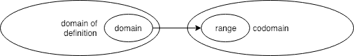
2.4.2.4. Functions are Three-Tuples
To completely specify a function, f, in a set-theoretical sense, we must identify three elements: its domain of definition, its codomain, and its set of ordered pairs, which will be some subset of the set of all possible ordered pairs formed from the values in its domain of definition and its codomain, respectively. Understood mathematically, then, a function, f, is what we can call a 3-tuple, f = (D, P, C), where D, a set of values, is the domain of definition of f; C, a set of values, is its codomain; and P, a set of ordered pairs of values from D and C, is single-valued. Our example function F can therefore be specified as  , where nat means the set of all natural numbers.
You can visualize this notation as specifying a domain of definition set on the left, a codomain set on the right, and as a set of ordered pairs in the middle, where each pair maps and element from the domain of definition on the left to an element in the codomain on the right. To be single-valued then means the no element on the left is ever connected to more than one element on the right.
From the set of ordered pairs of a function, we can infer its domain and range. The domain is the set of all values that appear in the first parts of any pair in P. The domain of F, is thus the set 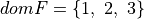 . The range of function is the set of values that appear in the second parts of any pair in P. The range of F is thus the set,
 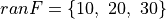 .
.
Note that two functions with different domains of definition and codomain sets are different functions, even if they have the same set of ordered pairs. For example, the function,  is not the same function as F because it has a different (smaller) domain of definition, even though its set of ordered pairs is the same as that of F.
2.4.2.5. Properties of Functions
The distinctions between the domain of definition of a function and its domain, and between its codomain and range, are vitally important when it comes to defining mathematically important properties of functions, as we will now see.
2.4.2.5.1. Total
We say that a function, f, is total if its domain is its entire domain of definition. A total function is defined for every element of its domain of definition. Another way to say this is that for any value, x, in the domain of definition of a function, f, there exists a value, y, in its codomain, such that y = f x. We can write this formally like this:
axioms S T : Type
def total(f: S → T) :=
      ∀(x: S), ∃(y: T),
          f x = y
Translating this logic into English one would say the following. Let S and T be sets. What it means for any function, f, with domain of definition, S, and codomain, T, to be total, is that for any value,  , there exists some value,
  , such that
  . In other words, for every value in the domain, S, of f, there is a corresponding value, which mathematicians call the image of that value under the function, f, in the codomain, T. As we will see later, in constructive logic, every value of a function type, , i.e., every lambda abstraction, represents a total function, but that is another matter.
2.4.2.5.2. Partial
A function that is not defined for every value in its domain of definition is said to be strictly partial. In this case, the domain of the function is a proper subset of (and thus is contained within but is not equal to) its domain of definition. In other words, a function is strictly partial if there exists some value, x, in its domain of definition for which there is no corresponding image, y, in the codomain.
Here’s how we can formalize this idea in mathematical logic:
axioms S T : Type
def strictly_partial(f: S → T) :=
    ∃(x: S), ¬∃(y: T),
        f x = y
In English, this says that for any function, f, with domain of definition, S, and codomain, T, f is strictly partial if there exists some such that there does not exist a , such that y = f x.
Our example function, F, is strictly partial in this sense. Its domain, { 1, 2, 3 }, is a proper subset of its domain of definition, which we defined to be the entire set of the natural numbers. That is, there is at least one value in its domain of definition for which there is no corresponding value in its codomain.
2.4.2.5.3. Terminology
In most mathematical writing, a total function is also considered to be a partial function. Under this conventional definition, every function is partial, while only some are total. In other writing, though less often, partial is taken to mean not total. In this class, we consider all functions, including total functions, to be partial, and use the term, strictly partial, to refer to functions that are not total. We also note that in some mathematical writing, the term, function, used by itself, is assumed to mean total function. As we will see later on in more detail, a “function” in constructive logic, i.e., a lambda abstraction, is inherently total. It must construct and return some value of its return (codomain) type for all values of its argument (domain-of-definition) type.
2.4.2.5.4. Surjective
We say that a function, f, is surjective if its range is its entire codomain. Mathematicians will also say that such a function is onto (shorthand for onto its entire codomain). Otherwise we say that f it is not surjective. In other words, a function is surjective if for any value, y, in its codomain, there exists some value, x, in its domain, such that y = f x. Said yet another way, every value, y, in the codomain of f, is the image, f x, of some value, x, in the domain of f.
We can now write this formally as follows:
axioms S T : Type
def surjective := ∀ f : S → T,
    ∀ y : T, ∃ x : S, f x = y
Our example function, F, is not surjective because there are values in the codomain that are not the images of any values in its domain. Only a few codomain values actually appear in any ordered pair in the function. If we had defined the codomain of F to be the set having only the values, 10, 20, and 30, then it would be surjective. One now sees why it is so important to be precise about the domains of definition, domains, codomains, and ranges of functions.
2.4.2.5.5. Injective
A function, f, is said to be injective if no two values in the domain of f have the same value in its range. Such a function is also said to be one-to-one, as opposed to being many-to-one. There are not many values in the domain that map to the same value in the range The set of ordered pairs of such a function contains no two pairs with different first (domain) elements and the same range element. We can represent this property formally as follows.
axioms S T : Type
def injective := ∀ f : S → T,
∀ x y : S, ∀ z : T,
    f x = z ∧ f y = z → x = y
2.4.3. Specifying Relations With Equations
Algebraic equations, such as  (or, equivalently, y = x) are often used to specify relations, in general, and functions, in particular. To be mathematically precise, when one writes such a specification, one must also identify the domain of definition and codomain of the function. So one would properly write something like this: “Let be a function with the domain of definition and codomain being the real numbers.” Or one might simply say, “Let f by the identity function on the real numbers.” In informal mathematical writing, mathematicians will often assume that readers understand the domains of definition and codomains of functions and so do not state them explicitly.
The function that an equation specifies is the set of all ordered pairs of values from the specified domain of definition and codomain that satisfy the given equation. Equations in this sense are predicates. When you fill in values for the variables, you get an equality proposition that either is or isn’t true. The given combination of variable values is in the relation if the resulting proposition is true, and is not in otherwise. So, again, when we say that a pair, (x, y) satisfies and equation, we mean that if the values in the pair are substituted for the variables in the equation, that the resulting equality proposition is made true. For example, the pair,  satisfies,
  , because 1 = 1 is true, and so does the pair,
  , but
, but  , does not, because the corresponding proposition, 1 = 2, is not true. That particular pair of values, (1, 2), doesn’t satisfy the predicate.
Not every equation specifies a function. For example, consider the equation  , where x and y range over the real numbers. (The set of real numbers is both the domain of definition and codomain of this function.) This equation is the equation of the unit circle in the real number plane. It is satisfied by both (0, 1) and (0, -1). Because there are two pairs in this relation with the same x value, the set of pairs satisfying it is not single-valued. This equation therefore does note specify a function. We use the term relation, rather than function, to refer to a set of ordered pairs that might or might not be single valued. In general, then, a function is a relation, namely one that is also single-valued, but not every relation is a function.
You can think of the property of being single-valued graphically. If you graph a relation, such as that given by the equation, (here the unit circle), and if you can draw a vertical line that crosses the graph at more than one point, the relation is not single valued and is not a function. In the example here, a vertical line through x = 0 will cross the circle at both y = 1 and at y = 1. The unit circle is thus a relation, and one that is satisfied only by certain pairs, but it is not a function because it’s not single valued.
2.4.4. Functions in Constructive Logic
In the lexicon of computer science, the word function is often used to mean a programming term (a piece of code if you will) that can be applied to an argument term to form an application term that can then be evaluated to compute a resulting value. Such a “function”, viewed as piece of code, is really another way to represent, or to specify, a function in a set theoretic sense. For example, the lambda abstraction, 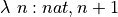 represents the function,
  , typically specified by the equation, f(x) = x + 1. Here we use what is called set comprehension notation to specify the set of all (x, y) pairs of natural numbers where the second is one more than the first. What is remarkable about lambda abstractions is that that they are not only specifications of functions, but they are also computable: they are programs that we can run to compute function values automatically with a digital computer.
The type of the argument to a lambda abstraction defines the domain of definition of the function that the lambda abstraction represents (here, nat). The return type is its codomain (here also nat). The the set of ordered pairs that the lambda abstraction represents is the set that would result by applying the lambda abstraction to each and every value in its domain of definition. We can call this set the extension of the function that is represented intentionally by the lambda abstraction.
One of the crucial properties lambda abstraction representations of functions in a constructive logic, such as that of the Lean Prover, is that all such functions are total. That is to say, they are defined for every element in their domain of definition. Such a “function” must be defined (return a result) for any value of its argument type. The Lean type checker will not accept a function definition that does not produce an answer for every value of its argument type. A lambda abstraction in Lean promises that for all values of its argument type, it can and, if asked, will construct and return a value of its result type.
2.4.4.1. Seeing the Totality of Functions in Constructive Logic
The totality of functions represented by lambda abstractions in the constructive logic of Lean is made clear by the following code, in which we define a function, f, to be of type  , and where we the function value is a lambda abstraction for the function that just increments its argument (adds one to it).
def f : ∀ n : ℕ, ℕ := λ n, n + 1
#check f
When we use #check to see what type Lean assigns to this function, it’s . Indeed, simply means in Lean. That means that for all argument values of type nat, such a function promises to produce a return value of type nat.
2.4.4.2. Representing Partial Functions in Constructive Logic
Representing strictly partial functions in a constructive logic will thus have to be done with something other than a lambda abstraction. As we will see later on, it has to be done with a declarative logical specification rather than with a computable lambda abstraction that can be applied to an argument and evaluated to produce a result automatically.
A consequence of this restriction is that one can apply any function (lambda abstraction) to any value of the specified argument type and get a result of the right type. Up to limits on the memory capacity of the computer on which a lambda abstraction application is evaluated, one will never get an error report, nor will a function application in a constructive logic ever go into an infinite loop. If one did go into an infinite loop, then it would never return a result and so would implement a strictly partial function. Without getting into reasons why, suffice it to say that this restriction is vital to preserving the consistency of the logic. If one were to allow infinite loops, one could construct a term of type false, i.e., a proof of false, and that would make the logic inconsistent, ruining its usefulness.
The restriction is necessary because Lean is not just a pure functional programming language but it is also a mathematical logic. Not every functional programming language imposes this restriction. An example of a functional language that does not impose such a restriction, and in which one can easily write code that goes into an infinite loop, or that produces errors even when applied to arguments of the right type, is Haskell. One can escape from this restriction in Lean using something called meta definitions. But if one does this, then one is no longer working in a logic with proof checking, but rather in a language like Haskell in which important forms of checking are no longer available.
As a concrete example, consider a function that takes two natural numbers, m and n and that returns the quotient, m/n. If written in Python or Java or C, one could apply the function to 7 and 0 as arguments, but one would then get a divide by zero exception (error report). No result would be returned. The arithmetic division function is partial (if its domain of definition is understood to be all pairs of natural numbers). In Lean, because division needs to return some result of the right type, for any expression of the form x/0, it just returns 0. This is not very satisfying. If one wants a better division function, it’s necessary to define the types of the arguments to be different, with the type of m being nat, but the type of n being what for now we might call “nat except for zero”. We are not prepared at this point to get into how one specifies such subtypes in constructive logic.
2.4.4.3. Some Examples to Consider
Here are a few simple examples of lambda abstractions in Lean that should now be easy to understand. As you review them, think carefully about how they are defined for all values of their argument types.
The first example gives two equivalent definitions of a function that returns double its natural number argument.
def double (n : ℕ) := 2 * n
def double' : ℕ →  ℕ := λ n , 2 * n

#check double
#check double'
#check double 3
#reduce double 3
#reduce double' 3
The second example gives two equivalent definitions of a function that returns the square of its natural number argument.
def square (n: ℕ) := n * n -- return type inferred
#check square
#check square 3
#reduce square 3

def square' : ℤ → ℤ := λ n, n * n

#reduce square' (-3)
Here’s a function that returns boolean true (tt) if a given natural number n is greater than or equal to zero and less than 2^32.
def uint32: ℕ → bool :=
λ n,
    if n >= 0 ∧ n < (pow 2 32) then tt else ff
#check uint32
Here’s a function that takes two natural number arguments and returns the value of the first raised to the power of the second.
def my_pow (x y: nat) := (pow x y)
#eval my_pow 2 16
2.4.5. Higher-Order Functions
In mathematics in general, and in functional programming languages, in particular, functions can be considered as values of function types. Functions can be named (bound to identifiers in Lean), and can be arguments to and results returned by other functions. Functions are values, too. An example familiar to anyone who has taken a course in differential calculus is the derivative operator, let’s call it D. It can now be understood as a kind of function that takes a function as an argument and yields a function as a result. For example, the derivative, D(f), of the function f(x) = x is the function, f’(x) = 1. Functions are values too isn’t such a crazy idea.
In functional programming, this concept is realized when one defines a function that either takes arguments or returns results of values whose types are function types. Our first example is of a function that takes a natural number as an argument and that returns a function that, when applied to any value, always returns that given number. This is a good example of a function that returns a function as a result.
def constNatFun (n: ℕ) : ℕ → ℕ := λ k, n
def f3 := constNatFun 3
#eval f3 17
Our second example is of a function that takes a function and a value as arguments and that applies the given function to the given argument to produce the result that is returned. This is a good example of a function that takes a function as an argument.
def apply (f: ℕ → ℕ) (n : ℕ) := f n

def square (n : ℕ) := n * n
def cube (n : ℕ) := n * n * n

#eval apply square 5
#eval apply cube 5
Our third example is of a function, compose, that takes two functions, f and g, and that returns a new function, namely the composition,  . This is the function that when applied to an argument, n, first applies f to n, and then applies g to that result. That is,
def compose (g: ℕ → ℕ) (f: ℕ → ℕ) (x: ℕ) : ℕ := g (f x)
#check compose

def double (n : nat) := 2 * n
def square (n : nat) := n * n

def sd := compose square double
def ds := compose double square

#reduce ds 5
#reduce sd 5
2.4.6. Exercises
- Is the function, G, that we defined above total? Explain.
- Give an example of a value in the domain of definition of our function, F, that proves that F is strictly partial, i.e., on which the function is not defined.
- Give an example of a value in the codomain of F that proves that F is not surjective.
- Is our example function, G, strictly partial? Explain.
- Identify a value in the codomain of F that is not the image of any value value in its domain of definition.
- Translate our logical definition of injective into mathematically precise English following the examples for other properties of functions given above.
- Is the function f(x) = log(x) over the real numbers injective? Is it surjective? Is it bijective? Explain each of your answers briefly.
- Is the relation,
 , single-valued? Explain your answer briefly.
 - Complete each of the following partial definitions in Lean by replacing the underscore characters to define a function of the specified types using lambda notation.
In preparation, please observe that if you hover your mouse over an underscore, Lean will tell you what type of term you is needed to fill that hole. Even more interestingly, if you fill in a hole with a term of the right type that itself has one or more remaining holes, Lean will tell you what types of terms are needed to fill in those holes! You can thus fill a hole in an incremental manner, refining a partial solution at each step until all holes are filled, guided by the types that Lean tells you are needed for any given hole.
def hw2_1: ℕ → ℕ :=
    λ(x: ℕ),
        _
def hw2_2: ℕ → ℕ → ℕ :=
    _
def hw2_3: (ℕ → ℕ) → (ℕ → ℕ) :=
    _
def hw2_4: (ℕ → ℕ) → (ℕ → (ℕ → ℕ)) :=
    _
def hw2_5: (ℕ → ℕ) → ((ℕ → ℕ) → (ℕ → ℕ)) :=
    _
2.5. Propositions
Having introduced terms (their types, including the definition and application of function terms), we turn to the second major category of expressions in predicate logic: the formulae. The formulae in predicate logic are symbolic expression called propositions and predicates. A propositions is read as asserting that a certain state of affairs holds in some domain. A predicate can be view as a proposition with parameters, with blanks to be filled in with particular values.
Specializing a predicate by giving specific values for its parameters yields a proposition. A proposition can also be thought of as a predicate with zero parameters. A predicate is said to be satisfied by a combination of parameter values if the resulting proposition is true in the given domain of discourse, and otherwise the predicate is said to be not satisfied by that combination of parameter values. A predicate can thus also be read as specifying the set of parameter value combinations that satisfy the predicate: that “make the resulting proposition true.”
In the constructive logic of Lean, a proposition is represented as a type. Proofs are values of such logical types. A predicates are represented as a function that take the parameters of the predicate as its arguments and that returns a corresponding proposition as a result. The rest of this chapter focuses on propositions. The next chapter focuses on predicates.
2.5.1. Natural Language
In a natural language, such as English, a proposition is just a declarative statement that we will interpret as asserting that some state of affairs holds in some domain of discourse (to be given by an interpretation). The declarative statement that “Jane is the mother of Tim” is an example of a proposition. We can form many such propositions. Here are some examples. Bob is Facebook friends with Mary. There is no largest natural number. There are no four integers, a, b, c, and n, where n > 2, such that  . If it rains outside, the streets will get wet. Jah walks to school or he carries his lunch. Zero equals one. False is true. War is Peace.
These are all perfectly good, though informally stated propositions. Whether any one of them is true depends on how we interpret the symbols, or names, that appear in these sentences. If by Jane and Tim we mean two specific people where the former person really is the mother of the latter, then we’d judge the proposition, Jane is the mother of Tim, to be true. If we interpret the symbols, Jane and Tim, differently, e.g., as referring to people in a different family, then the same proposition might well turn out to be false.
2.5.2. Syntax and Semantics
We see in this example a fundamental distinction: between the syntax of propositions, or their form, and their semantics, or their meaning, and in particular whether they are true or not under some particular interpretation of the symbols that they contain. Syntax is about the valid forms of propositions. Semantics is about deciding whether any given proposition is true or not.
Now some propositions are true no matter how one interprets the symbols that they contain. For example, if P is some proposition, then the proposition P and not P is always false, as it can never be the case in reality that some state of affairs prevails and also does not prevail at the same time. For example, under any reasonable laws of reasoning, it can’t be that Jane is Tim’s mother and Jane is not Tim’s mother, or that x equals y and x does not equal y. Such propositions are logical contradictions, and are thus necessarily false, no matter how we interpret the symbols they contain.
As another example, if P and Q are propositions, and we know that P and Q is true, then we can infer that P is true. The reason is that to know that the proposition, P and Q, is true is to know that each of P and Q is true individually. We could express this proposition a bit more formally by saying, “if the proposition P and Q is true then the proposition P is true.” We could be even more precise by writing it formally, as  .
.
2.5.3. Valid Reasoning
In this class, and in most any class that teaches logic, we focus on forms of propositions whose meanings, or truth values, do not depend on the interpretations under which they are evaluated. The truth of Jane is the mother of Tim depends on what we mean, how we interpret, the symbols Jane, Tim, and is mother of. But P and not P is false no matter what we mean by P.
In particular, we will focus on establishing and using valid rules, with different rules for different forms of propositions. The aim, and the essence of symbolic logic, is that all reasoning then can be done syntactically, without a need to think about interpretations. That is, we aim to establish universally valid principles for reasoning about the truth or falsity of various forms of propositions. As an example, we’ve already said that for any proposition, P, the proposition P and not P is false. This is an example of a universal reasoning principle: a contradiction is always false, no matter how we interpret P.
2.5.4. Forms of Propositions
Here we introduce the various forms of propositions in constructive and predicate logic, and how we will interpret these forms of propositions independent of the details of the meanings of the symbols they contains. The first segment of this course introduces each form of proposition and valid principles for reasoning about propositions of these forms.
Here’s Lean code showing briefly each form of propositions. To get set up, we assume that P and Q are arbitrary propositions; T is an arbitrary type; t1 and t2 are terms of this type; and Pred is a predicate (addressed in detail in the next chapter) on values of this type. Given this set-up, we then introduce the forms of propositions in predicate logic. The #check commands show that each term is of type Prop, which is to say, “it’s a proposition.”
axioms (P Q : Prop)
axioms T: Type
axioms (t1 t2 : T)
axiom Pred : T → Prop

#check true
#check false
#check P
#check Q
#check t1 = t2
#check P ∧ Q
#check P → Q
#check P ↔ Q
#check P ∨ Q
#check ¬ P
#check ∀ t : T, Pred t
#check ∃ t : T, Pred t
Todo
fix quotation
From Avigad’s TPIL: “The order of operations is as follows: unary negation ¬ binds most strongly, then ∧, then ∨, then →, and finally ↔. For example, a ∧ b → c ∨ d ∧ e means (a ∧ b) → (c ∨ (d ∧ e)). Remember that → associates to the right (nothing changes now that the arguments are elements of Prop, instead of some other Type), as do the other binary connectives. So if we have p q r : Prop, the expression p → q → r reads “if p, then if q, then r.” This is just the “curried” form of p ∧ q → r.”
2.5.4.1. True
In Lean and in predicate and constructive logic, generally, is a proposition.
#check true
We intend true to be a proposition that is always true. We thus define it as a type, a logical type, that has at least one value, one proof. In fact, it is defined as a type with exactly one value, and that value is given the name, intro. The name is defined in the namespace of the type, true, and so is referred to as . The proposition, , is trivially provable, therefore uninteresting, and seldom seen in practical work in logic.
example : true := true.intro
This small block of Lean code uses the example keyword in Lean to check an anonymous proof. It’s like def but without giving a name. It’s purpose is simply to type check a term to confirm (or not) that it’s of a specified type. Here the type is the proposition, true. The value, i.e., the proof, is true.intro. And the Lean type checker accepts true.intro as a value (a proof!) of the logical type, of the proposition, true.
2.5.4.2. False
In Lean and in predicate and constructive logic, generally, , is also a proposition.
#check false
The proposition, false, is meant always to be false. A proposition is false in a constructive logic if no proof of it can ever be produced. Lean thus defines this proposition as a logical type that has absolutely no values whatsoever: no proofs. Viewed as a type, false is uninhabited. One can never prove this proposition to be true, because to do that would require a proof and this type is defined as having no values at all.
The proposition, false, appears often in practical work. The reason why is that, if we wish to prove that some proposition is false, we will often do so by showing that if we assume that it is true, by assuming that there is a proof of it, then we’d be able to construct a proof of false. Since that is impossible, it must be that no proof of the proposition exists, so the proposition must be false. The assumption that one can be given a proof of the proposition must be in error and so we can conclude that it’s not true. This style of argument, this proof strategy is called proof by negation.
2.5.4.3. Conjunction
If P and Q are any two propositions, then  is also a proposition. It is pronounced P and Q.
axioms (P Q: Prop)
#check P ∧ Q
We call such a proposition a conjunction. We call the constituent propositions, P and Q, conjuncts. We intend such a proposition to assert that P is true and Q is true.
To enforce this meaning, the natural deduction system of logical reasoning defines just one proof constructor, one introduction rule, called and.intro. It is defined to take a proof, p, of P, and a proof, q, of Q, as arguments. It then returns a proof of . Because this is the only rule for building a proof of , in this logic there is simply no way to prove unless one already has proofs of the individual conjuncts. In this way, the limited availability of basic inference rules enforces the intended meaning of the logical connective, .
A proof of , in turn, can be understood as simply being a pair of the constituent proofs, <p, q>, that type checks as a term of type . This proof term is just a certain kind of data structure, a pair, <p, q>, with a certain type, . Proofs in constructive logic are computational objects!
Going the other way, given a proof of , from it one can derive each of the individual proofs, a proof p of P and a proof, q, of Q, by projecting out the left or right elements of the pair <p,q>.
Once again, the inference rules of the logic enforce the intended meaning of the connective. Here we can say that if we’re given a proof that is true, then we can immediately deduce that P is true, and we can obtain a proof of it; and the same goes for Q.
2.5.4.4. Implication
If P and Q are any two propositions, then  is also a proposition.
axioms (P Q: Prop)
#check P → Q
We call such a proposition an implication. It can be pronounced as P implies Q.” It it intended to mean that, *if P is true then Q is true. In a logic in which for P or Q to be true means we have a proof of P or Q, then for such an implication proposition to be true, it must be that if one can be given a proof of P then one can construct a proof of Q.
To prove a proposition of this form, one must show that if one assumes that P is true, which in Lean means that if one assumes that one has a proof of P, then one can build a proof of Q. Such a proof is then a function: one that if given a proof of P as an argument, returns a proof of Q. The existence of such a function proves that the implication is true.
The truth of such an implication, however, does not mean that P is necessarily true. It might be impossible ever to give a proof of P that such a function could then turn into a proof of Q. it just means that if you assume that P is true, e.g., that a proof of P is given as an argument to a function, then based on that assumption, one can produce a proof of Q.
In the other direction, if one has, or assumes one has, a proof of , and if one also has, or assumes one has, a proof of P, then by applying the proof of (a function!) to the proof of P, what one gets in return is a proof of Q. If any proof of P can be turned into a proof of Q, then it must be the case that if P is true then so is Q. That is what it means for an implication to be true.
As we will will see, one proves such an implication precisely by producing a function that has type : a function that shows that if there actually is a proof of P to which the function can be applied, then a proof of Q can be built. A proof of an implication is a function, a recipe, for converting any proof of P, if one even exists, into a proof of Q.
The connection between computation and logic in constructive logic grows increasingly clear. We now also see the importance of lambda abstraction-defined functions being total: to prove that P implies Q we need a function that can convert any proof of P (if one exists) into a proof of Q.
2.5.4.5. Equivalence
If P and Q are any two propositions, then  is also a proposition.
axioms (P Q: Prop)
#check P ↔ Q
It can be pronounced as P is equivalent to Q or P if and only if Q. In constructive logic, it asserts that “if you have a proof of P (showing that P is true), then you can derive a proof of Q (showing that Q is true as well); and if you have a proof of Q then you can derive a proof of P.” In other words, if either P or Q is true, then both are; so if either is false, then both must be, as well.
EXERCISE: Write a truth table for this connective.
One can now see that really just means  . To prove a proposition of this form, one must therefore have two proofs, one showing that P implies Q, and the other showing that Q implies P. In the other direction, from a proof of P if and only if Q, one can derive a proof of P implies Q and also a proof of Q implies P.
2.5.4.6. Disjunction
If P and Q are any two propositions, then  is also a proposition.
axioms (P Q: Prop)
#check P ∨ Q
We pronounce it as “P or Q”. We call such a proposition a disjunction, and the constituent propositions, P and Q, disjuncts. We interpret such a disjunction as asserting that at least one of P or Q is true. While having a proof of tells us that at least one of the disjuncts is true, it does not tell us which one.
EXERCISE: Is it true that, for any propositions, P and Q, that  ? Is it true that
  ?
?
To prove such a disjunction, we need either a proof of P or a proof of Q. That much establishes that at least one of the disjuncts is true, making the whole disjunction true. Going the other way, if we already have a proof of , the best we can do with it is to show that no matter which of the two disjuncts is true, the truth of some other proposition, R, follows.
To use a proof of , we thus also need proofs of  and of
  . If we have these proofs then from a proof of , the truth of R must follow, because it follows whether P or Q is true because P is true or because Q is true. In either case, R will also be true.
2.5.4.7. Negation
If P is a proposition, then ~P is also a proposition. We pronounce it as “not P”. We mean it to assert that P is false, which is to say not true. To show that a proposition, P, is false, we show that if we assume it is true, that there is a proof of it, then we can then derive a proof of false. Since there is no proof of false, the assumption that P is true must have been wrong, thus proving that P is false. In the other direction, if we have a proof of ~P, then if in some context we can also obtain a proof of P, then we can apply the proof of ~P to the proof of P to obtain a proof of false, proving that there a contradiction has arisen. Because contradictions cannot arise in a consistent logic, this shows that we made an incorrect assumption somewhere, and that the situation can safely be ignored.
2.5.4.8. Predicates
At this point we take a detour to quickly introduce the notion of predicates. A predicate is a proposition with parameters, or placeholders. When you give values for the parameters of a predicate, it reduces to a proposition, sometimes called an atomic formula. For example, 5 = 0 is a proposition, but n = 0, where n is a parameter, is a predicate. You get a different proposition for each value of n that you use to fill in the blank. If n is 5, you get the proposition 5 = 0. If n is 27, you get the proposition 27 = 0. If n is 0, you get the proposition, 0 = 0. Predicates give rise to families of propositions, some of which might be true (one is in our case), and others of which might not be.
In constructive logic, predicates are formalized as functions. A predicate is a function that takes values for one or more parameters, and that reduces to a proposition. We represent the predicate in the preceding example as the function 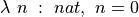 . Applying it to the value, 5, using the expression,
 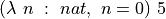 , would yield the proposition, 5 = 0. We will usually bind a name to a predicate so that we don’t have to type lambda expressions. For example, we might bind the name isZero to the predicate, i.e., to the function, . Having done so, we can write the proposition that 5 = 0 using the expression, isZero 5.
The type of a predicate in constructive logic, then, is a function type: from whatever types of value the predicate takes as its argument or arguments, to Prop. A predicate, given values for all of its arguments, reduces to a proposition. One can now see that a predicate is a generalized (parameterized) proposition, and a proposition is a fully reduced predicate (with zero remaining parameters).
Check it out in the following logic, in Lean. Lean confirms the informal account we’ve given here. Line one and two compare and contrast a proposition and a predicate. Specializing the predicate by applying it to a specific value returns a proposition, also sometimes called an atomic formula in writing on logic. Lines 3 through 6 show that we can apply the predicate to the value, 5, to get back to the proposition on line 1. Lines 7 and 8 give examples of a few of the many other propositions we can obtain by applying the predicate to other values. Finally, we show that while we cannot prove some of the resulting propositions (because they’re just not true), we can prove one: we can prove the proposition, isZero 0. Indeed, 0 is the only value that satisfies the predicate: for which the resulting proposition has a proof.
def isZeroFive : Prop     :=       5 = 0
def isZero     : ℕ → Prop :=  λ n, n = 0

#check isZeroFive
#check isZero
#check isZero 5

#reduce isZeroFive
#reduce isZero 5
#reduce isZero 27
#reduce isZero 16
#reduce isZero 0

example : isZero 27 :=
    _   -- stuck!
example : isZero 0 := rfl
EXERCISE: Extend the Lean code here to #check the types of, and the values that result, when isZero is applied to a few other argument values. Use it to represent the proposition that zero equals one hundred. Finally, use it to state, and then prove, the proposition that one minus one equals zero.
2.5.4.9. Universal Quantification
If P is any type and Q is any formula, whether a proposition or a predicate, then  is a proposition. We call such a proposition a universally quantified proposition. Typically Q is a predicate taking an argument of type P.
What we mean for such a proposition to assert is that for any value, p, of type P, the predicate, Q, is true. That is, the proposition obtained by substituting any value, p, for the argument of Q is true. As a simple example, the proposition, 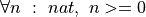 asserts that any natural number n is greater than or equal to zero. This is a true proposition.
To prove that a proposition, , is true, we assume that we have some arbitrary but specific value, p, of type P and show that in the context of this assumption, we can derive a proof of Q. Going the other direction, if we have a proof of , and we have some specific value, p of type P, then we can apply the proof of to that specific value to obtain a proof of Q. A proof of thus acts like a function, converting values of type P into proofs of Q.
2.5.4.10. Existential Quantification
If P is any type and Q is any formula, whether a proposition or a predicate, then  is a proposition. We call such a proposition an existentially quantified proposition. Typically Q is a predicate taking an argument of type P.
What we mean for such a proposition to assert is that there is *some value, p, of type P, for which the predicate, Q, is true. As an example, the proposition, 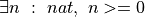 asserts that there is some natural number n that is greater than or equal to zero. This is a true proposition.
To prove a proposition, , in a constructive logic, one must produce some specific value, p, which we call a withness, along with a proof that Q is true for that specific value. Going the other direction, if one has a proof of , then one can give a name to that object that is proven to exist and one can derive a proof that that named thing makes the predicate, Q, true.
2.5.5. EXERCISES
Stay tuned!
2.6. Predicates
A predicate is a proposition with parameters. When one fills in the formal parameters of a predicate with actual values of suitable types, the result is a proposition. A proposition thus can be seen as a special case of a predicate, namely as a predicate with zero parameters. Conversely, a predicate can be seen as a generalized proposition: one that can be specialized to any of a number of propositions by giving values for the parameters.
2.6.1. Two Examples
Let’s start with a proposition: “Marilyn is the Mother of Kevin.” There are no blanks, no parameters, to fill in here. By replacing the actual values, Marilyn and Kevin, with parameters, or “blanks”–let’s call them M and C (for mother and child)–we obtain a predicate: M is the mother of C. Logicians typically use an abbreviation for the name of the predicate, and put the arguments after the name, thus: isMotherOf M C. This is a predicate: a proposition with parameters.
If we fill in actual values for M and C, e.g., with the names, Jane and Tim, then we get a proposition, Jane is the mother of Tim (isMotherOf Jane Tim). If we fill in M and C with different names, Maya and Andrew, we get a different proposition: isMotherOf Maya Andrew.
Predicates thus give us a way to form whole families of propositions without having to write each one individually. A proposition can be seen as a predicate with no more parameters to be filled in. Logicians also call propositions atomic formulae.
As we will see in this chapter, we formalize predicates as functions that take values, e.g., the names, Jane and Tim, or Maya and Andrew, as arguments, and that return propositions, i.e., terms of type Prop, as results.
This code block briefly illustrates the idea. See the code. An explanation follows.
axiom Person : Type
axioms (Marilyn Kevin Maya Tim Andrew Jane : Person)
axiom isMotherOf : Person → Person → Prop
#check isMotherOf Marilyn Kevin
axiom marilynIsMotherOfKevin : isMotherOf Marilyn Kevin
theorem itIsTrue: isMotherOf Marilyn Kevin := marilynIsMotherOfKevin
We axiomatically declare Person to be a type and Marilyn, Kevin, Maya, Time, Andrew, and Jane to be values (terms) of this type. Next we axiomatically declare isMotherOf to be a predicate that takes two people as arguments. In the next line, we use #check to confirm that when we apply this predicate/function to two values of type Person the resulting term is a proposition: a value of type Prop. In the final line we axiomatically delare marilynIsMotherOfKevin to be a proof of the proposition, isMotherOf Marilyn Kevin, which, of course, we assert that Marilyn is the Mother of Kevin. We’ve thus built a little logical model of a small world with some people in it in which one, Marilyn, is the mother of another, Kevin.
Consider another example. Suppose a predicate, fromCharlottesville p, has a parameter, p, and we intend that when it is applied to a particular person, p, we mean for the resulting proposition to be interpreted as asserting that the person named by p really is from Charlottesville.
When an actual argument value, such as Kevin, is given for p, then the placeholder(s) in the predicate where p occurs are filled in with that value,yielding a proposition about that particular individual. Here, the resulting proposition is fromCharlottesville Kevin. This is a proposition that will want to interpret as asserting that Kevin really is from Charlottesville. The proposition, fromCharlottesville Mary gives rise to a different proposition, which we would read as asserting that Mary is from Cville.
For each possible value of p, there is a corresponding proposition, fromCharlottesville p. A predicate thus gives rise to a family of propositions, one for each argument value.
2.6.2. Satisfaction
Not every proposition derived by applying a predicate to one or more arguments will be true. Rather, a predicate in effect picks out argument values that are said to satisfy the predicate, by giving rise to a family of propositions, some of which are true, i.e., for which proof are available.
In our simple example, perhaps it really is true that Kevin is from Charlottesville but Mary is not. We would say that the choice of Kevin as the value of the parameter, p, satisfies the predicate, because there is a proof of the resulting proposition, while the choice of Mary does not. This predicate then, in a sense, picks out the members of a set: the set of all objects having the property that the predicate represents. Here, that is the property of being from Charlottesville.
2.6.3. Predicates are Functions
In Lean, we represent a predicate as a function that takes one or more more arguments and that returns a proposition. One must reason separately about whether any proposition formed in this way is true or not. In any case, such a proposition is generally “about” its arguments, in that argument values usually become parts of the resulting proposition. As examples, “fromCharlottesville Kevin” makes a claim about Kevin (that he is from Cville), and “fromCharlottesville Mary” makes a similar claim, but now it’s about Mary.
A predicate has a type. Because it’s a function in constructive logic, it has a function type. A predicate returns some proposition, which itself is some value of type Prop. So the return type of a predicate is always Prop. The type of a predicate is thus the type of a function its argument type (or types) to Prop. In the preceding example, if Kevin and Mary are values of some type, Person, then the predicate, fromCharlottesville, will be represented as a function from Person to Prop, and its type would therefore be  .
.
The following example formalizes our informal example in Lean, adding an assumed proof of the proposition that Kevin is from Charlottesville, but not adding one for Mary. This bit of code we interpret as describing a certain state of affairs in the world: that there is a person, Kevin, from Charlottesville, and a person, Mary, not from Charlottesville.
axioms (Person: Type) (Kevin Mary: Person)
axiom fromCharlottesville: Person → Prop
#check fromCharlottesville Kevin
#check fromCharlottesville Mary
axiom kevinIsFromCville: fromCharlottesville Kevin
2.6.4. Properties
As we see here, a predicate can be used to specify a property of values in some domain. In constructive logic, a domain is a type. In this case, it’s Person. So we can understand fromCharlottesville as specifying the property, attributable to a Person, of being from Charlottesville. Every Person, p, who satisfies the predicate (for which the resulting proposition has a proof and is thus true) can be said to have the property, while everyone else lacks the property.
The concept of properties is vitally important in computer science, mathematics, logic. Let’s consider some other examples. Being odd, being even, being prime, are all properties of natural numbers. Being tall is a property of people. Being raining is a property of the weather outside at the present moment. Having an infinite loop is a property of programs.
In computer science, we are particularly interested in properties of things like problems that computers might solve, such as whether they’re solvable by a computer at all. This is the property of being computable. Whether an algorithm solves a problem in an amount of time given by a polynomial function of the size of the input is a property of algorithms.
The rest of this section expands on the idea that predicates specify properties with a series of examples.
2.6.4.1. Being even
Consider a predicate, isEven n, that is meant to specify the property of a natural number being even. Given a specific value for n, say 3, this predicate would give a proposition, in this case isEven 3, that we interpret as asserting that 3 is even.
For our predicate to properly capture our intended interpretation, this particular proposition must must have no proof, as 3 is not even. On the other hand, even 4, isEven 6 and even 8, among many other resulting propositions, must be true. That is, there must be proofs for these propositions, and for all propositions that result when even is applied to a natural number that really is even.
To this end, we have to define isEven in such a way that every proposition it produces for even inputs has a proof, and every proposition that it produces for odd inputs does not. One way to do this is to have it produce propositions that assert that n mod 2 = 0. That is, we can define evenness in terms of the mod 2 arithmetic function, which takes a value, n, and returns n mod 2. This value is the remainder when one takes the quotient of n and 2. If this number is 0, then n is even. If it’s 1, then n is not even. We thus define isEven as a function that takes a natural number, n, as an argument, and that returns the proposition, (n % 2 = 0). We will be able to prove such a proposition whenever n really is even, and we won’t be able to prove it whenever n is odd.
Here’s our isEven predicate in Lean. The first line defines isEven n as a predicate. The second line shows that the result of applying it to 3 is a proposition. The fourth line shows what proposition that is: namely that 3 % 2 = 0. This proposition is of course false. The next two lines show that isEven 4 is also a proposition, and what proposition it is. In this case, the resulting proposition is true as long as the modulus operator is defined in the usual way, which it is in Lean. What this means is that we should be able to prove the proposition, isEven 4, and that is exactly what we do on the last line.
def isEven (n :ℕ) : Prop := nat.mod n 2 = 0
#check isEven       -- it's a predicate
#check isEven 3
#reduce isEven 3
#check isEven 4
#reduce isEven 4
lemma fourIsEven : isEven 4 := eq.refl 0
You can think of (eq.refl 0) as the application of a function, eq.refl, defined in Lean’s libraries, to a natural number, 0, returning a proof of 0 = 0, and Lean accepts that as a proof of the proposition that 4 % 2 = 0 because Lean reduces 4 mod 2 to 0, meaning that what is to be proved is simply that 0 = 0, which is true.
This isEven predicate picks out the set of even numbers, in the sense that it generates a family of propositions, where all the ones about even numbers are true, and all the others are not. In a sense that we will make precise in the section on set theory, this predicate can be said to specify the set of even numbers. We can think of it as a membership predicate for this set, expressing the property of being in the set of even numbers. Every even natural number has this property, and every other number does not.
2.6.4.2. Being equal to zero
We can formalize the property of a natural number being equal to zero. Here’s this predicate formalized as a function in Lean.
def isZero (n : ℕ): Prop := (0 = n)
lemma zeroIsZero: isZero 0 := eq.refl 0
2.6.4.3. Unsatisfiable
A predicate, isFalse, that always returns the proposition, false, cannot be satisfied by any argument, because every argument value leads to false, which has no proof. Such a predicate is said to be unsatisfiable. An unsatisfiable predicate specifies the empty set of values of its argument type.
def isFalse (n : ℕ) : Prop := false
2.6.4.4. Trivial
A predicate, isTrue, that always returns the proposition, true, for any argument value, is satisfied by every argument value, because the proposition true always has a proof. Such a predicate specifies the set of all values of its argument type. We leave it to the reader to implement this predicate for natural numbers, and then to implement a polymorphic version that applies to values of any type. (EXERCISE.)
2.6.5. Relations
In the last subsection, properties, we discussed how predicates with one argument can be understood as specifying properties of values of their argument types. As such, a predicate with one argument can also be read as specifying a set of values: those values that satisfy the predicate, i.e., that have the specified property. The isEven predicate, for example, can be taken to specify the set of even natural numbers.
Predicates can also have multiple arguments. In this case, a given combination of argument values will or will not satisfy a given predicate. So we can think of such a predicate as specifying a property of tuples (ordered pairs or triples or other combinations) of argument values. Such a predicate can be seen as specifying a set of tuples: all tuples (combinations) of values of the argument types that satisfy the predicate. Mathematicians call such a set of tuples a relation.
As an example, and as a brief preview of the next chapter, we can consider equality as a predicate, and as a binary relation: one involving pairs of values. We say that the arity of such a relation is 2. In Lean this relation is called eq. It takes two arguments, such as m and n, both of the same type (more about this later), and returns a proposition that we read as asserting that the two values are equal. For example, the term, eq 3 4, the application of the eq predicate two two values, yields a proposition asserting that 3 = 4. Indeed, in Lean, we can write this proposition as 3 = 4, and that is just a nice notation for eq 3 4.
2.6.5.1. Exercises
- Which of the following predicates is true for all values of its argument type? Which is true for no values of its argument type?
def is_absorbed_by_zero(n: ℕ): Prop := n * 0 = 0
def equals_self_plus_one(n: ℕ): Prop := n = n + 1
- Here is a definition of a data type with the names of the seven days of the week as values. Given this datatype, define a predicate, funday d, in Lean that expresses the property of being a fun day. Define it so that a day, d, is fun if and only if d is between Thursday and Saturday, inclusive. Then write and prove a lemma claiming that Saturday is a fun day.
inductive day : Type
| Monday : day
| Tuesday : day
| Wednesday : day
| Thursday : day
| Friday : day
| Saturday : day
| Sunday : day
- Define wahoo, of type Prop, to be a proposition that asserts that every day is fun.
- Define, wah, of type Prop, to be a proposition that asserts that there is at least one fun day.
- Define a predicate, isSquare, that expresses the relation between two natural numbers that the second natural number is the square of the first and prove that the pair, (3, 9), is in the isSquare, relation. Explain in English what set of values this predicate specifies.
6. In lean, the function, string.length, returns the length of a given string. Define a predicate, sHasLenN, taking a string and a natural number as arguments that asserts that a given string has the given length. Write the function using lambda notation to make the function type of the predicate explicit in its definition. Briefly explain the nature of each string-nat ordered pair in the relation that this predicate defines.
- A Pythagorean triple is a 3-tuple of natural numbers such that the sum of the squares of the first two is equal to the square of the third. Define a predicate, PyTri, on three arguments of type nat that is satisfied by any, and only by a, Pythagorean triple. Then use example to assert that the combination of values, 3, 4, 5, is Pythagorean, leaving the proof to be filled in as a hole (using an underscore).